Decomposition and Smoothing Methods

The reference text for this chapter is from Penn State University.
Decomposition
In the previous chapters, differencing would be applied whenever we observe a mean trend or seasonal pattern. In this chapter we will learn another method – decomposition procedures – to extract the trend and seasonal factors in a time series using nonparametric detrending. Some more extensive decompositions might include long-run cycles, holiday effects, day of week effects etc.
One of the main objectives for a decomposition is to estimate seasonal effects that can be used to create and present seasonally adjusted values. A seasonally adjusted value removes the seasonal effect from a value so that trends can be seen more clearly.
Basic structures
We’re going to consider the following two structures for decomposition models:
Additive model:
$$ X_t = T_t + S_t + I_t = \text{Trend} + \text{Seasonal} + \text{Random} $$
Multiplicative model:
$$ X_t = T_t S_t I_t = \text{Trend} \times \text{Seasonal} \times \text{Random} $$
Here the random component is denoted $I_t$ because it’s often called irregular in software.
The additive model is useful when the seasonal variation is relatively constant over time, whereas the multiplicative model is useful when the seasonal variation changes (increases) over time. This is because if we log-transform both sides of the multiplicative model, it becomes an additive model with a log-transformed series:
$$ \log X_t = \log T_t + \log S_t + \log I_t $$
So when the variance is not constant over time, we can either apply a multiplicative model, or transform the series first and then apply an additive model. The latter approach is more flexible as it’s not limited to a log-transformation.
Steps in decomposition
Estimation of the trend. Two approaches with many variations of each are:
- Smoothing techniques such as
moving averages - Regression
- Smoothing techniques such as
Removal of the trend. The de-trending step is different for additive and multiplicative models:
- Additive: $X_t - \hat{T}_t$
- Multiplicative: $X_t / \hat{T}_t$
Estimation of seasonal components from the de-trended series. The seasonal effects are usually adjusted so that they average to 0 for an additive decomposition, or average to 1 for a multiplicative decomposition.
The simplest method for estimating these effects is to average the de-trended values for a specific season. For example, we average the de-trended values for all Januarys in the series to get the seasonal effect for January.
Determination of the random (irregular) component.
- Additive: $\hat{I}_t = X_t - \hat{T}_t - \hat{S}_t$
- Multiplicative: $\hat{I}_t = \frac{X_t}{\hat{T}_t \times \hat{S}_t}$
The remaining $\hat{I}_t$ part might be modeled with an ARIMA model. Sometimes steps 1 to 3 are iterated multiple times to get a stationary process. For example, after step 3 we could return to step 1 and estimate the trend based on the de-seasonalized series.
Let’s say our times series can be decomposed into
$$ X_t = f(t) + W_t $$
where $f(t)$ is a deterministic trend and $W_t$ is stationary. Our goal is to remove $f(t)$ from $X_t$.
If we take a parametric approach, we may assume some form of the deterministic trend such as
$$ f(t) = \beta_0 + \beta_1 t \text{ or } \beta_0 + \beta_1 t + \beta_2 t^2 $$
and the only thing we need to do is to estimate the $\beta$’s.
In our nonparametric approach1, we estimate $f(t)$ directly at $t$. This is obviously more flexible as we don’t have to make assumptions on the form of $f(t)$, but it comes with the caveat of being less efficient as we have to estimate $f(t)$ for each point of $t$. We also can’t write out the formula of $f(t)$ explicitly – we get $\hat{f}(t)$ instead.
Some popular nonparametric methods are kernel smoothing (LOWESS), splines, and wavelets. The kernel usually requires a larger sample size and the target function to be smooth. Splines are better with smaller sample sizes in higher dimensions, and wavelets are better with data that are discontinuous or contain spikes.
Decomposition in R
The decompose() function in R can be used for both additive and multiplicative models. The type parameter can be specified as "additive" or "multiplicative". Note that the seasonal span for a series needs to be defined using the freq parameter in the ts() function.
The following example uses the dataset of quarterly beer production in Australia from 1956 to 1973. Data for the first 18 years are used to demonstrate the functions. The series looks like this after additive decomposition2:
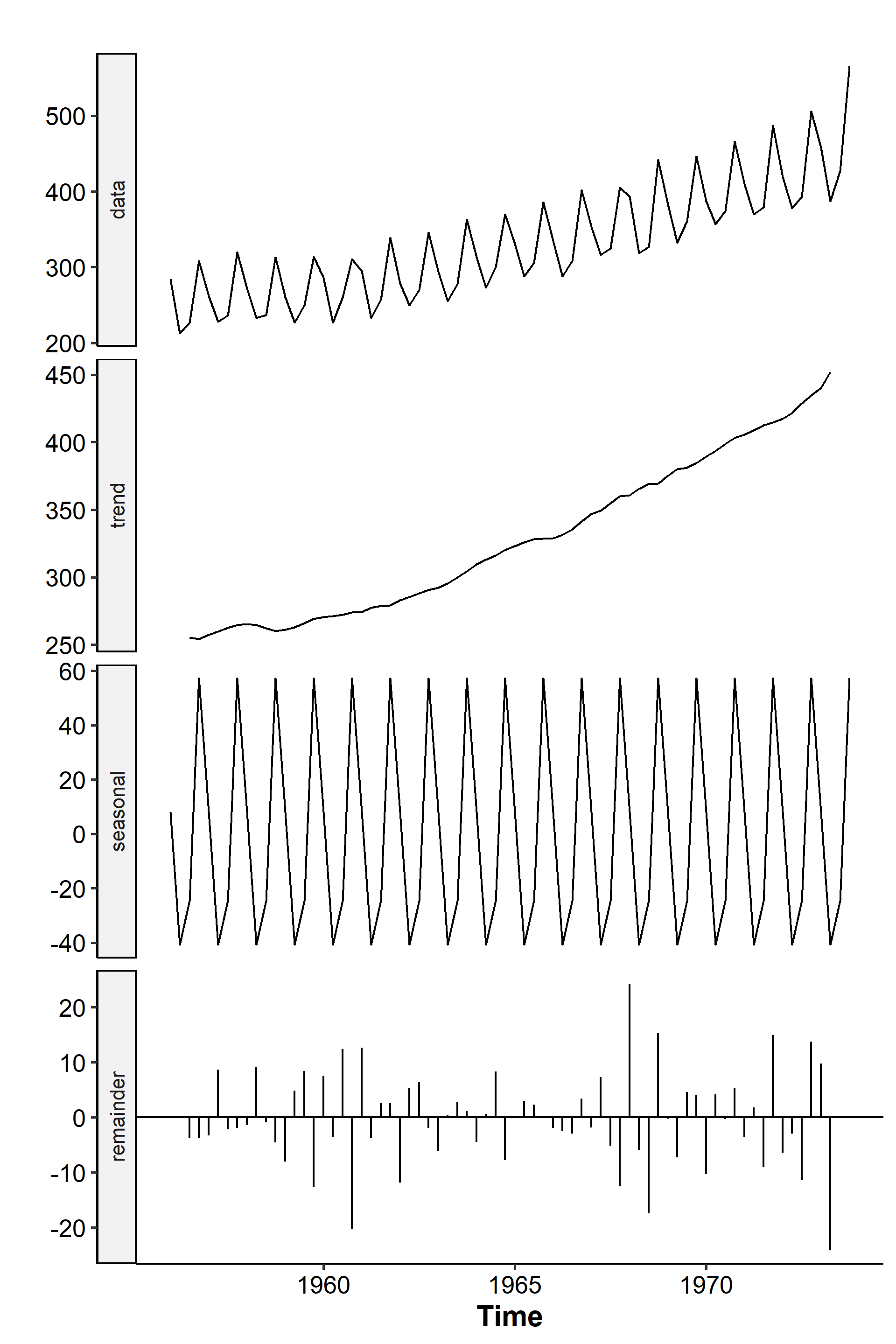
The function plots the original data, the mean trend, the seasonal component, and the remainders3. See that the seasonal component stays constant for each quarter and is a regularly repeating pattern. We can also set the type parameter to “multiplicative” and get:

Smoothing
Smoothing is used to help us better see patterns in time series. Generally we try to smooth out the irregular roughness to get a cleaner signal. For seasonal data, we might also smooth out the seasonality so that the trend could be identified. Smoothing doesn’t provide us with a model, but it can be a good step in describing various components of a series.
The term filter is sometimes used to describe a smoothing procedure. For example, if the smoothed value for a particular time is calculated as a linear combination of the observations for surrounding time points, it might be said that we’ve applied a linear filter to the data.
Moving average
As we said earlier, a simple but effective method to estimate the trend is the moving average. For example, the trend values in the Australian beer example were determined as centered moving averages with length 4 (because there are four quarters per year). For time $t=3$, we first average the observed data values at times 1 to 4:
$$ \frac{1}{4} (X_1 + X_2 + X_3 + X_4) $$
Then the average of the values at times 2 to 5:
$$ \frac{1}{4}(X_2 + X_3 + X_4 + X_5) $$
Then we take the average of these two values to get
$$ \frac{1}{8}X_1 + \frac{1}{4}X_2 + \frac{1}{4}X_3 + \frac{1}{4}X_4 + \frac{1}{8}X_5 $$
We’re doing this because the length is an even number. For length 5, we can simply take
$$ \frac{1}{5}(X_1 + X_2 + X_3 + X_4 + X_5) $$
More generally, the centered moving average for time $t$ of a quarterly series is
$$ \frac{1}{8}X_{t-2} + \frac{1}{4}X_{t-1} + \frac{1}{4}X_t + \frac{1}{4}X_{t+1} + \frac{1}{8}X_{t+2} $$
and for a monthly series:
$$ \frac{1}{24}X_{t-6} + \sum_{j=-5}^5 \frac{1}{12}X_{t+j} + \frac{1}{24}X_{t+6} $$
The decompose() function uses this method (symmetric window with equal weight), and we can get the results with decomp_beer_add$trend. See how we have two NA values at the beginning and at the end because the moving average can’t be calculated at these time points. This linear filter can be calculated manually in R using:
| |
Other variations of the moving average exist and may serve different purposes. For example, to remove a seasonal effect, we may calculate the moving average with a length equal to the seasonal span. We may only use the previous $n$ time points, i.e. the one-sided moving average:
$$ \frac{1}{4}(X_t + X_{t-1} + X_{t-2} + X_{t-3}) $$
In R, this can be found by
| |
Lowess
Another more advanced decomposition method is the locally weighted scatterplot smoothing (LOWESS)4. To understand what this is, we need to introduce the concept of kernel smoothing.
In the simplest univariate case where $X_1, \cdots, X_n \overset{i.i.d.}{\sim} f_X$, our goal is to estimate the density function $f_X$. In parametric density estimation, we assume some density function (e.g. Binomial, Poisson, Normal, etc.) and estimate the parameters, often with MLE.
Parametric density estimation is efficient when the assumptions on the distribution are met. In nonparametric density estimation, we estimate $\hat{f}_X(x)$ at a given $x$ without assuming a form of the distribution. At the expense of efficiency, we gain a lot of flexibility.
The histogram is a naive approach of density estimation, although an obvious disadvantage is that it’s discrete and not smooth. It also depends on the bin width $b$ and the starting point. Kernel density estimation is proposed to overcome some of these problems.
Let $h$ be the bandwidth. We can express the density estimate at $x$ of the histogram as
$$ \begin{aligned} \hat{f}_X(x) &= \frac{\text{Frequency}}{nb} \\ &= \frac{\text{number of }X_i \in (x-h, x+h)}{2nh} \\ &= \frac{\sum_{i=1}^n I(X_i \in (x-h, x+h))}{2nh} \\ &= \frac{1}{2nh}\sum_{i=1}^n I\left( |x - X_i| < h \right) \\ &= \frac{1}{2nh}\sum_{i=1}^n I\left( \left|\frac{x - X_i}{h}\right| < 1 \right) \end{aligned} $$
The discreteness comes from the indicator function. The idea of kernel density estimation is instead of this indicator function, we plug in a smoother kernel function $K$ that assigns larger weights for points closer to $x$ and lower weights for distant points:
$$ \hat{f}(x) = \frac{1}{2nh}\sum_{i=1}^n K\left( \frac{x - X_i}{h} \right) $$
For the bivariate case where we have $n$ pairs of observations $(X_1, Y_1)$, $\cdots$, $(X_n, Y_n)$ with
$$ Y_i = f(X_i) + \epsilon_i, \quad \epsilon_i \overset{i.i.d.}{\sim} N(0, \sigma^2) $$
where $f(X_i) = E(Y_i \mid X_i)$ is an unknown regression function. Kernel smoothing works similarly to kernel density estimation. In the simplest form, we take the weighted average of neighboring points to $x$:
$$ \hat{f}(x) = \sum w_i (x, h) Y_i $$
Some popular choices are local linear regression, local polynomial regression, and local constant regression.
In R, we can use the stl() function to apply seasonal decomposition on a time series by Lowess. Afterwards, the seasadj() function could be used to get seasonally adjusted data.
| |
We can also combine this with the forecast package to model the remainder with an ARIMA, exponential smoothing, just the previous observation (naive), or a random walk:
| |
Exponential smoothing
SARIMA used differencing to take care of the trend, but the components aren’t really extracted. The decomposition methods extract the mean and seasonal trends and models the remainder.
The technique soon to be introduced is for short-run prediction only, altough it’s called a smoothing method.
Single exponential smoothing
In single (or simple) exponential smoothing, it’s assumed a time series could be decomposed into the following model
$$ X_t = T_t + I_t $$
where $T_t = \beta_{0, t}$ is a linear trend that’s locally constant, and $I_t$ is the remainder. The basic forecasting equation is often given as
$$ \ell_{t+1} = \alpha X_t + (1-\alpha)\ell_t, \quad 0 \leq \alpha \leq 1 $$
We forecast the value of $X$ at time $t+1$ to be a weighted combination of the observed value at time $t$ and the forecasted value at time $t$. $\alpha$ is called the smoothing constant, and 0.2 is the default value for multiple programs for some mysterious reason.
A relatively small $\alpha$ value means our one-step ahead forecast depends mostly on the previous prediction. If the series changes very quickly, then we may consider increasing $\alpha$ since the previous value doesn’t help much with the next one.
We can expand the recursive formula above to get
$$ \begin{aligned} \ell_{t+1} &= \alpha X_t + (1-\alpha)[\alpha X_{t-1} + (1-\alpha)\ell_{t-1}] \\ &= \alpha X_t + \alpha(1-\alpha)X_{t-1} + \alpha(1-\alpha)^2 X_{t-2} + \cdots + \alpha(1-\alpha)^{t-1}\ell_1 \end{aligned} $$
where the initial value $\ell_1$ is either $X_1$ or $\sum_{t=1}^T X_t / T$. The method is called exponential smoothing because the weight is exponentially decreasing as we move back in the series. The prediction at $t=T$ for $h$ lags after is simply
$$ \hat{X}_{T+h} = \ell_T, \quad h = 1, 2, \cdots $$
By now you may have noticed the relationship between this simple exponential smoothing and ARIMA models – in fact, this method is equivalent to the use of an ARIMA(0, 1, 1) model:
$$ X_t - X_{t-1} = Z_t + \theta Z_{t-1} \Rightarrow X_{t+1} = X_t + Z_{t+1} + \theta Z_t $$
If we set $Z_{t+1} = X_{t+1} - \hat{X}_{t+1}$, i.e. express it as the forecasting error term, then
$$ \begin{aligned} \hat{X}_{t+1} &= X_{t+1} - Z_{t+1} \\ &= X_t + \theta Z_t \\ &= X_t + \theta(X_t - \hat{X}_t) \\ &= (1 + \theta) X_t - \theta \hat{X}_t \\ &= \alpha X_t + (1-\alpha)\hat{X}_t \end{aligned} $$
Due to this equivalence, we can just fit an ARIMA(0, 1, 1) model to the observed dataset and use the results to determine the value of $\alpha$. This is “optimal” in the sense of choosing the best $\alpha$ for the observed data.
In R, the forecast::ses() function could be used for simple exponential smoothing. We can specify alpha = 0.2 and initial = "simple" to get the procedure described above. If initial is set to optimal, then the initial value is optimized along with the smoothing parameter.
Double exponential smoothing
The limitations with simple exponential smoothing is that it can’t deal with trends beyond linear. In double (or linear) exponential smoothing, a slight nonlinear trend could be handled:
$$ X_t = T_t + I_t $$
where $T_t = \beta_{0, t} + \beta_{1, t} t$ is locally linear. This method may be used when there’s trend but no seasonality.
Instead of using a single smoothing constant, this method combines exponentially smoothed estimates of the trend (slope $\beta_{1, t}$) and the level (intercept $\beta_{0, t}$). The forecast equation, also known as Holt-Winters forecasting, is
$$ \hat{X}_{t+1} = \ell_t + b_t $$
where
$$ \begin{gathered} \ell_t = \alpha_t + (1-\alpha)(\underbrace{\ell_{t-1} + b_{t-1}}{\hat{X}t}), \quad 0 \leq \alpha \leq 1 \\ b_t = \beta(\ell_t - \ell{t-1}) + (1- \beta)b{t-1}, \quad 0 \leq \beta \leq 1 \end{gathered} $$
The smoothed level is more or less equivalent to a simple exponential smoothing of the data, and the smoothed trend is somewhat like a simple exponential smoothing of the first differences.
The initial values are $\ell_1 = X_1$ and $b_1 = X_2 - X_1$, or they can be obtained through simple linear regression:
$$ (\hat{\alpha}, \hat{\beta}) = \arg\min_{\alpha, \beta} SSE(\alpha, \beta) $$
where the SSE is
$$ SSE(\alpha, \beta) = \sum_{t=1}^T (X_{t+1} - \ell_t - b_t)^2 $$
The prediction at $t=T$ for $h$ lags is
$$ \hat{X}_{T+h} = \ell_T + b_T \times h, \quad h = 1, 2, \cdots $$
The procedure is equivalent to fitting an ARIMA(0, 2, 2) model. In R, the forecast::holt() function can be used. The parameters are very similar to the ones given in ses(), with an additional beta parameter.
Seasonal exponential smoothing
The model for seasonal exponential smoothing adds another component to simple exponential smoothing:
$$ X_t = T_t + S_t + I_t $$
where $T_t = \beta_{0, t}$ is locally constant. The basic forecast equation is
$$ \hat{X}_{t+1} = \ell_t + s_{t+1-p} $$
where $p$ is the seasonal period, and
$$ \begin{gathered} \ell_t = \alpha(X_t - s_{t-p}) + (1-\alpha)\ell_{t-1} \\ s_t = \beta(X_t - \ell_t) + (1-\beta)s_{t-p} \end{gathered} $$
$\ell_t$ is the weighted average of the de-seasonalized observation and the previous prediction. $s_t$ is the weighted average of the de-trended observation and the previous seasonal component.
The prediction at $t=T$ for $h$ lags is
$$ \hat{X}_{T+h} = \ell_T + s_{T-p+h} \times h, \quad h = 1, 2, \cdots $$
This method is equivalent to ARIMA$(0, 1, p+1) \times (0, 1, 0)_p$. It’s not of much practical use as it cannot handle nonlinear trends.
Holt-Winters seasonal exponential smoothing
A much more flexible method is Holt-Winters seasonal exponential smoothing. The additive model is
$$ X_t = T_t + S_t + I_t, \quad T_t = \beta_{0, t} + \beta_{1, t} t \text{ (locally linear)} $$
and the basic forecast equation is
$$ \hat{X}_{t+1} = \ell_t + b_t + s_{t+1-p} $$
where
$$ \begin{gathered} \ell_t = \alpha(X_t - s_{t-p}) + (1-\alpha)(\ell_{t-1} + b_{t-1}), \quad 0 \leq \alpha \leq 1 \\ b_t = \gamma(\ell_t - \ell_{t-1}) + (1-\gamma)b_{t-1}, \quad 0 \leq \gamma \leq 1 \\ s_t = \delta(X_t - \ell_t) + (1-\delta)s_{t-p}, \quad 0 \leq \delta \leq 1 \end{gathered} $$
Prediction at time $t=T$ for $h$ lags is
$$ \hat{X}_{T+h} = \ell_T + b_T \times h + s_{T_p+h}, \quad h = 1, 2, \cdots $$
This method is equivalent to an ARIMA$(0, 1, p+1) \times (0, 1, 0)_p$ model.
We can also consider a multiplicative model when the variance increases over time:
$$ X_t = T_t \times S_t \times I_t, \quad T_t = \beta_{0, t} + \beta_{1, t}t $$
The basic forecast equation is
$$ \hat{X}_{t+1} = (\ell_t + b_t)s_{t+1-p} $$
where the intercept, slope and seasonal components are
$$ \begin{gathered} \ell_t = \alpha \cdot \frac{X_t}{s_{t-p}} + (1-\alpha)(\ell_{t-1} + b_{t-1}) \\ b_t = \beta (\ell_t - \ell_{t-1}) + (1-\beta)b_{t-1} \\ s_t = \gamma \cdot \frac{X_t}{\ell_t} + (1-\gamma)s_{t-p} \end{gathered} $$
and the prediction at $t=T$ for $h$ lags is
$$ \hat{X}_{T+h} = (\ell_T + b_T \times h)s_{T_p+h}, \quad h = 1, 2, \cdots $$
In R, the forecast::hw() function can be used, setting seasonal to “additive” or “multiplicative” for the two models above.
The “nonparametric” here doesn’t mean distribution-free. It’s referring to the literal meaning of not having parameters. ↩︎
R code for generating the figure:
↩︎1 2 3 4 5 6 7 8 9 10 11 12 13 14library(tidyverse) library(forecast) theme_set( ggpubr::theme_pubr() + theme( axis.title = element_text(face = "bold", size = 14) ) ) data("ausbeer", package = "fpp") beerprod <- window(ausbeer, end = c(1973, 4)) decomp_beer_add <- decompose(beerprod, type = "additive") autoplot(decomp_beer_add, range.bars = F)The word “remainder” is used rather than “random” because maybe it’s not really random! ↩︎
For a more in-depth introduction to Lowess, see this chapter in the Nonparametric Methods course. ↩︎
| Nov 17 | Spectral Analysis | 9 min read |
| Oct 13 | Seasonal Time Series | 17 min read |
| Oct 09 | Variability of Nonstationary Time Series | 13 min read |
| Oct 05 | ARIMA Models | 9 min read |
| Sep 30 | Mean Trend | 13 min read |