Conditional Heteroscedastic Models

This final chapter in on a type of model that’s popular within financial time series. The source of most of the material is listed here.

In our previous chapters, we used transformation to take care of changing variances over time, but the transformations were global and can’t deal with local changes. In fields like finance where those local changes are often of interest, conditional heteroscedastic models can be used to model volatility.

In finance, volatility is interpreted as the risk, and it’s the standard deviation of the underlying asset returns. In a classical regression setting, we would have an i.i.d. model in the form of

$$ X_t = \mu + \sigma\epsilon_t, \quad \epsilon_t \sim N(0, 1) $$

In our previous homogeneous time series, we allow the mean to change over time:

$$ X_t = f(X_{t-1}, X_{t-2}, \cdots) + \sigma\epsilon_t, \quad \epsilon_t N(0, 1) $$

In heteroscedastic time series, we further allow the standard deviation $\sigma$ to vary over time:

$$ X_t = f(X_{t-1}, X_{t-2}, \cdots) + g(X_{t-1}^2, X_{t-2}^2, \cdots) \epsilon_t, \quad \epsilon_t \sim N(0, 1) $$

Volatility

The volatility is the variance in a time series conditional on past data. In finance, the option price, foreign currency market, risk management, and asset allocation are all affected by volatility. Volatility modeling provides a simple approach to calculate the VaR in risk management. A risk measure is an estimate for the amount of capital to be held in reserve for a given financial position with a given level of risk to insure against substantial losses. VaR is simple and can be easily interpreted as it’s a quantile of the loss distribution.

$$ VaR_\alpha(L) = \inf\{ l \in \mathbb{R}: F_L(l) \geq \alpha \} $$

where $F$ is the CDF of the loss function, and the confidence level of the VaR is $1-\alpha$. In other words, the VaR is defined as the potential loss in the worst case scenario at $1-\alpha$ confidence level.

Modeling the volatility of a time series can improve the efficiency in parameter estimation and the accuracy in interval forecast.

Characteristics of volatility

• Volatility is not directly observable.
• Volatility may be high for certain time periods, and low for other periods. This is called volatility clustering.
• Volatility evolves over time in a continuous manner. That is, volatility jumps are rare.
• Volatility seems to react differently to a big price increase or a big price drop. There’s usually less volatility in a big price increase, because people want to hold on to the stocks longer. This is called the leverage effect.

ARCH effect

In finance, the data studied are usually log returns:

$$ r_t = \log(1 + R_t) = \log \frac{P_t}{P_{t-1}} = \log(P_t) - \log(P_{t-1}) $$

The ARCH effect states that the log returns are serially uncorrelated or have minor lower-order autocorrelations. However, the squared log returns are serially correlated. We’ll use The S&P 500 closing prices from 2013 to 2015 as an example.

1
2
3
4
5
6

library(quantmod)

getSymbols("^GSPC", from = "2013-01-02", to = "2015-12-31")
price <- GSPC$GSPC.Close
log_price <- log(price)
log_return <- diff(log_price)[-1]  # drop first NA element

With our experience, this looks like a stationary time series, although there appears to be some increased variances towards the end. Let’s check the ACF of the log returns (mean part) and the squared log returns (variance part).

As we can see in Figure 2, there’s more serial correlation in the squared log return.

Volatility models

The conditional mean and variance are

$$ \begin{gathered} \mu_t = E[r_t \mid \mathcal{F}_{t-1}] \\\sigma_t^2 = Var(r_t \mid \mathcal{F}_{t-1}) = E[(r_t - \mu_t)^2 \mid \mathcal{F}_{t-1}] \end{gathered} $$

where $\mathcal{F}_{t-1}$ denotes the information set available at time $t-1$, i.e. past data up to $X_{t-1}$. The ARMA$(p, q)$ models for the conditional mean is

$$ r_t = \mu_t + a_t, \quad \mu_t = \phi_0 + \sum_{i=1}^p \phi_ir_{t-i} + \sum_{i=1}^q \theta_ia_{t-i} $$

Then, the remaining part (the conditional variance) is modeled as

$$ \sigma_t^2 = E\left[(r_t - \mu_t)^2 \mid \mathcal{F}_{t-1} \right] = E\left[ a_t^2 \mid \mathcal{F}_{t-1} \right] = Var(a_t \mid \mathcal{F}_{t-1} ) $$

Volatility models are concerned with the evolution of $\sigma_t^2$. In general, $a_t$ is referred to as the shock or innovation. The models for $\mu_t$ and $\sigma_t^2$ are referred to as the mean and volatility equations for $r_t$, respectively.

Let’s take a look at a different (longer) time period of the S&P 500 data. There’s some big spikes in the middle, so volatility models might be used to account for the variance changes.

When we look the the ACF and PACF for the mean model of the log returns, it seems there are two spikes in both the ACF and the PACF, so we could consider AR(2), MA(2) and ARMA(1, 1) as candidate models.

We could try fitting an MA(2) model:

 1
 2
 3
 4
 5
 6
 7
 8
 9
10
11
12

m <- arima(log_return, order = c(0, 0, 2))
m

# Call:
# arima(x = log_return, order = c(0, 0, 2))

# Coefficients:
#          ma1      ma2  intercept
#       0.0374  -0.0502      3e-04
# s.e.  0.0081   0.0081      1e-04

# sigma^2 estimated as 9.414e-05:  log likelihood = 49362.59,  aic = -98717.17

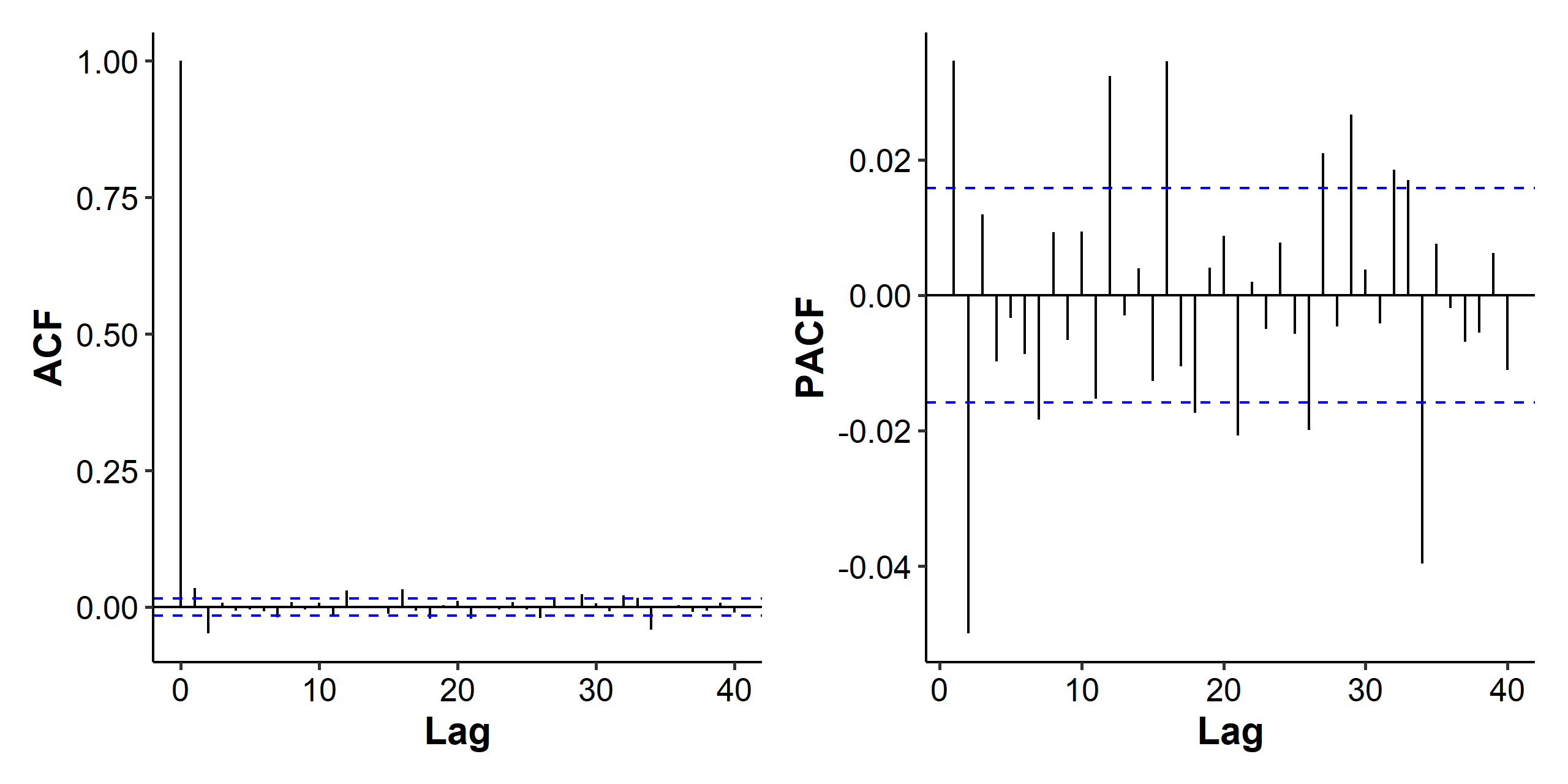
The intercept seems small enough for us to go for a zero-mean model, but let’s not worry about that for now. We then check the ACF and PACF of the residuals and squared residuals, i.e. the $a_t$ part, to see if there’s a need for modeling the volatility part.

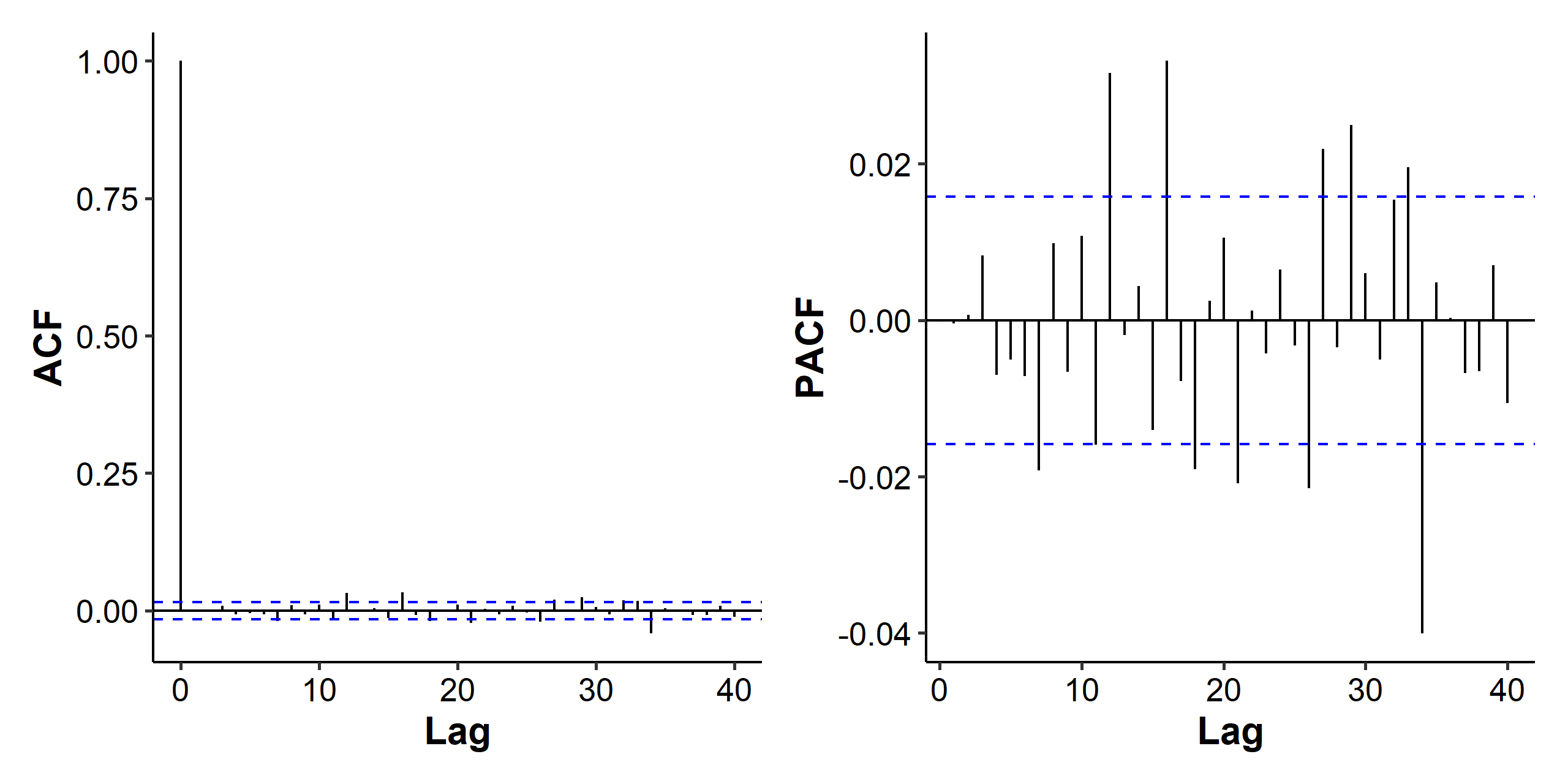
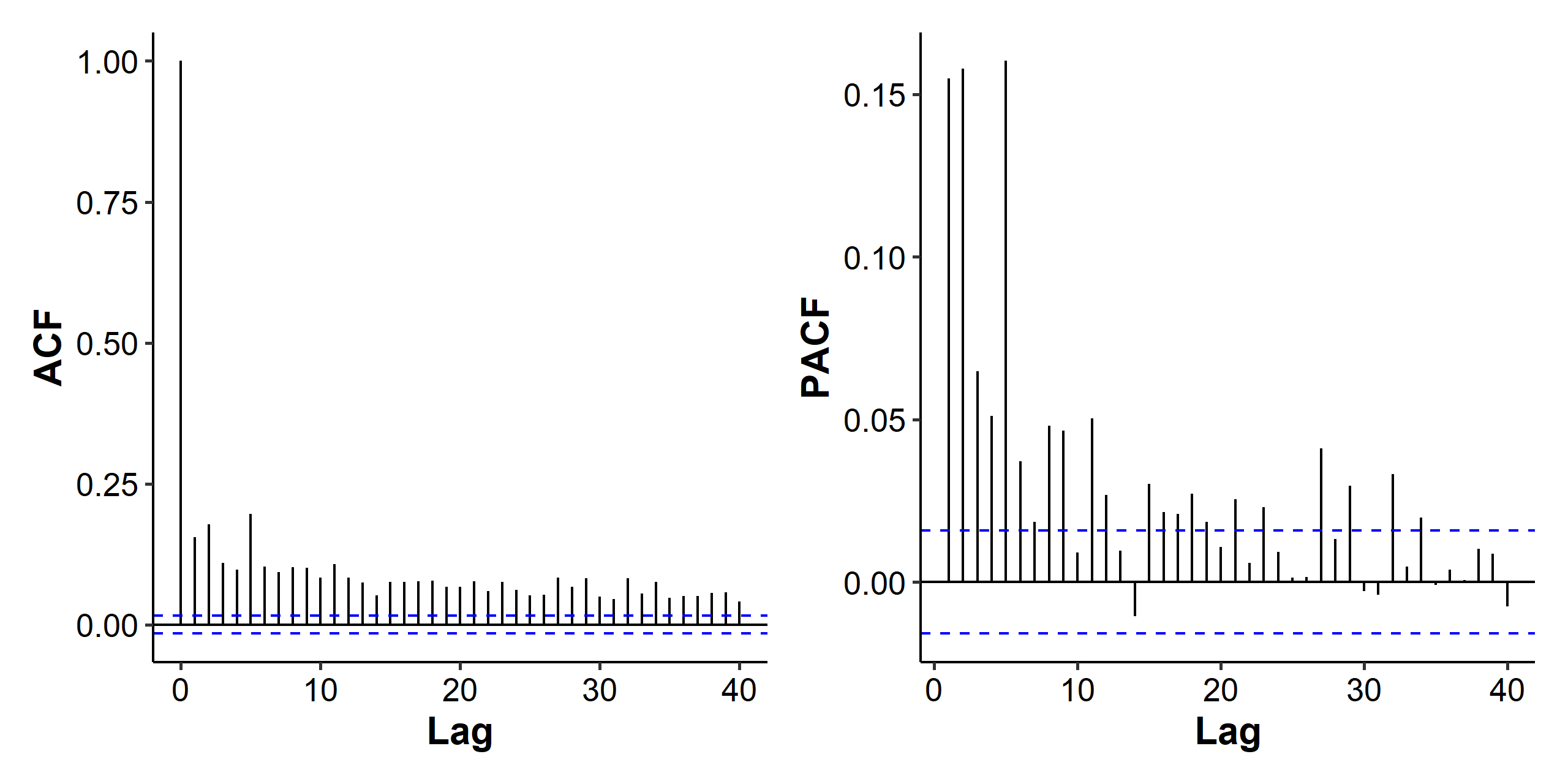
The spikes in the later lags of the PACF indicate that the model for the mean part ($\mu_t$) could be improved. As for the ACF and PACF of the squared residuals, we can see strong autocorrelation, which indicates the volatility is not constant over time and should be modeled.

The correlation we found in the mean part could also be affected by the volatility changes. The ARCH effect is somewhat obvious, but we can also use the Ljung-Box test on the squared residuals and conclude that there is serial correlation.

1
2
3
4
5
6

Box.test(residuals(m)^2, lag = 5, type = "Ljung-Box", fitdf = 3)

# 	Box-Ljung test

# data:  residuals(m)^2
# X-squared = 1780.1, df = 2, p-value < 2.2e-16

Steps of building a model

1. Test for serial dependence in the data, i.e. check the ACF and PACF of the series.
2. Build an model for the series to remove any linear dependence if necessary. This corresponds to the mean part of the model.
3. Test for ARCH effects by using the residuals of the mean equation.
4. Specify a volatility model if ARCH effects are statistically significant, and perform a joint estimation of the mean and volatility equations.
5. Check and refine the fitted model.

To test for ARCH effects, let $\tilde{a}_t = r_t - \tilde\mu_t$ be the residuals of the mean equation. The squared residual series $\hat{a}_t^2$ is then used to check for the ARCH effect using the Ljung-Box test.

ARCH model

We’ve mentioned ARCH multiple times now, but what is it? The Autoregressive Conditional Heteroscedasiticity model of order $m$ assumes that

$$ a_t = \sigma_t\epsilon_t, \quad \sigma_t = \alpha_0 + \alpha_1 a_{t-1}^2 + \cdots + \alpha_m a_{t-m}^2 $$

where $\alpha_0 > 0$ and $\alpha_i \geq 0$ for $i > 0$. $\epsilon_t$ is a sequence of i.i.d. random variables with mean 0 and variance 1. In practice, $\epsilon_t$ is often assumed to follow a standard normal or standardized student-$t$ distribution¹.

From the structure of the model, it can be seen that large past squared shocks $\{a_{t-i}^2\}_{i=1}^m$ imply a large conditional variance $\sigma_t^2$ for the innovation $a_t$. Consequently, $a_t$ tend to be assumed a large value if the previous volatility is large.

Under the ARCH framework, large shocks tend to be followed by another large shock. This feature is similar to the volatility clustering observed in asset returns.

Properties of ARCH(1)

The model is

$$ a_t = \sigma_t \epsilon_t, \quad \sigma_t^2 = \alpha_0 + \alpha_1 a_{t-1}^2 $$

where $\alpha_0 > 0$ and $\alpha_1 \geq 0$. The unconditional mean of $a_t$ is

$$ \begin{aligned} E[a_t] &= E\left[ E[a_t \mid \mathcal{F}_{t-1}] \right] = E\left[ E[\sigma_t \epsilon_t \mid \mathcal{F}_{t-1}] \right] \\ &= E\left[ \sigma_t E[\epsilon_t \mid \mathcal{F}_{t-1}] \right] = E[\sigma_t E[\epsilon_t]] \\ &= 0 \end{aligned} $$

The unconditional variance of $a_t$ is

$$ \begin{aligned} Var(a_t) &= E[a_t^2] = E\left[ E[\sigma_t^2 \epsilon_t^2 \mid \mathcal{F}_{t-1}] \right] \\ &= E\left[ \sigma_t^2 E[\epsilon_t^2] \right] = E[\alpha_0 + \alpha_1 a_{t-1}^2] \\ &= \alpha_0 + \alpha_1 Var(a_{t-1}) \end{aligned} $$

If $a_t$ is a weakly stationary process², then $Var(a_t) = Var(a_{t-1})$, which yields

$$ Var(a_t) = \frac{\alpha_0}{1 - \alpha_1}, \quad 0 \leq \alpha_1 \leq 1 $$

Weakness of ARCH models

1. Positive and negative shocks have the same effects on volatility. In practice, it’s well known that the price of a financial asset responds differently to positive and negative shocks.
2. ARCH model with Gaussian innovation is not good enough for capturing excess kurtosis of a financial time series. Skewed and $t$-distributions are often used.
3. Lower-order (small $m$) ARCH models often don’t perform well, and we end up with a lot of parameters to estimate in order to model the volatility. This led to the development of GARCH models.
4. The ARCH model does not provide any new insight for understanding the sources of variation of a financial time series.

Building an ARCH model

1. Order determination. If the ARCH effect in the residuals is significant, we can use the ACF and PACF of $a_t^2$ to determine the ARCH order.

   The characteristics of PACF of AR models can be used, i.e. counting the number of spikes starting from lag 1. We can also use the AIC/BIC to determine the order.

2. Estimation using conditional MLE.

   • Under the normality assumption, the conditional likelihood function is

     $$ \begin{aligned} f(a_{m+1}, \cdots, a_T \mid \boldsymbol{\alpha}, a_1, \cdots, a_m) &= \prod_{t=m+1}^T f(a_t \mid \mathcal{F}{t-1}) \\ &= \prod{t=m+1}^T \frac{1}{\sqrt{2\pi\sigma_t^2}} \exp\left( -\frac{a_t^2}{2\sigma_t^2} \right) \end{aligned} $$

     where $\boldsymbol{\alpha} = (\alpha_0, \cdots, \alpha_m)$ and $\sigma_t^2$ can be evaluated recursively.

   • Under the $t$-distribution, it’s assumed that

     $$ \epsilon_t = \frac{x_\nu}{\sqrt{\nu / (\nu - 2)}} $$

     where $x_\nu$ is a Student $t$-distribution with $\nu$ degrees of freedom. Then the conditional likelihood function is

     $$ f(a_{m+1}, \cdots, a_T \mid \boldsymbol{\alpha}, A_m) = \prod_{t=m+1}^T \frac{\Gamma\left(\frac{\nu + 1}{2}\right)}{\Gamma\left(\frac{\nu}{2}\right) \sqrt{(\nu-2)\pi}} \cdot \frac{1}{\sigma_t}\left( 1 + \frac{a_t^2}{(\nu-2)\sigma_t^2} \right)^{-\frac{\nu+1}{2}} $$

     where $\nu > 2$ and $A_m = (a_1, \cdots, a_m)$.

3. Model diagnostics.

   • For a properly specified ARCH model, the standardized residuals behave as a sequence of i.i.d. random variables:

     $$ \tilde\epsilon_t = \frac{a_t}{\sigma_t} $$

   • Check ACF and perform Ljung-Box test of the squared residuals $\{\tilde\epsilon_t^2\}$.

   • Under the normality assumption (which is often not true), check the Q-Q plot and perform the Jarque-Bera test of the residuals.

4. Forecasting. The point forecast of $a_{h+1}$ is the conditional variance

   $$ \hat\sigma_h(1) = Var(a_{h+1} \mid \mathcal{F}_h) = \alpha_0 + \sum_{i=1}^m \alpha_i a_{h+1-i}^2 $$

   The 2-step ahead forecast is

   $$ \hat\sigma_h(2) = Var(a_{h+2} \mid \mathcal{F}_h) = \alpha_0 + \alpha_1\hat\sigma_h(1) + \sum_{i=2}^m \alpha_i a_{h+2-i}^2 $$

   In general, the $l$-step ahead forecast is

   $$ \hat\sigma_h(l) = \alpha_0 + \sum_{i=1}^m \alpha_i \hat\sigma_h(l-i) $$

Model fitting in R

The fGarch package could be used to fit ARCH (and later GARCH) models. The input data are the raw log returns, not the residuals or squared residuals. For ARCH models, we set the second parameter of garch() to 0.

 1
 2
 3
 4
 5
 6
 7
 8
 9
10
11
12
13
14
15
16
17
18
19
20
21
22
23
24
25
26
27
28
29
30
31
32
33
34
35
36
37
38
39
40
41
42
43
44
45
46
47
48
49

m <- garchFit(formula = ~ garch(1, 0), data = log_return, trace = F)
summary(m)
# Title:
#  GARCH Modelling

# Call:
#  garchFit(formula = ~garch(1, 0), data = log_return, trace = F)

# Mean and Variance Equation:
#  data ~ garch(1, 0)
# <environment: 0x000002863be9e240>
#  [data = log_return]

# Conditional Distribution:
#  norm

# Coefficient(s):
#         mu       omega      alpha1
# 4.2733e-04  6.3858e-05  3.3075e-01

# Std. Errors:
#  based on Hessian

# Error Analysis:
#         Estimate  Std. Error  t value Pr(>|t|)
# mu     4.273e-04   7.038e-05    6.072 1.27e-09 ***
# omega  6.386e-05   9.852e-07   64.816  < 2e-16 ***
# alpha1 3.308e-01   1.571e-02   21.051  < 2e-16 ***
# ---
# Signif. codes:  0 ‘***’ 0.001 ‘**’ 0.01 ‘*’ 0.05 ‘.’ 0.1 ‘ ’ 1

# Log Likelihood:
#  50352.15    normalized:  3.280911

# Standardised Residuals Tests:
#                                 Statistic p-Value
#  Jarque-Bera Test   R    Chi^2  45483.73  0
#  Shapiro-Wilk Test  R    W      NA        NA
#  Ljung-Box Test     R    Q(10)  77.8096   1.347256e-12
#  Ljung-Box Test     R    Q(15)  95.02417  1.135758e-13
#  Ljung-Box Test     R    Q(20)  103.5256  2.930989e-13
#  Ljung-Box Test     R^2  Q(10)  2654.464  0
#  Ljung-Box Test     R^2  Q(15)  3486.78   0
#  Ljung-Box Test     R^2  Q(20)  4055.941  0
#  LM Arch Test       R    TR^2   1738.581  0

# Information Criterion Statistics:
#       AIC       BIC       SIC      HQIC
# -6.561432 -6.559938 -6.561432 -6.560937

The fitted model above is

$$ r_t = \mu_t + a_t = 4.2733 \times 10^{-4} + a_t,\quad \sigma_t^2 = 6.3858 \times 10^{-5} + 0.33075 a_{t-1}^2 $$

In the Standardised Residuals Tests part, the Jarque-Bera test and Shapiro-Wilk test are tests for normality. The Ljung-Box tests are grouping the time points into blocks, and testing for autocorrelation within the blocks. R stands for residuals and R^2 for squared residuals. It seems there’s still strong serial correlation within the standardized residuals, so we may have to increase the order of the ARCH model.

In the garchFit() function, we can also specify the cond.dist parameter to some other conditional distribution, such as snorm for skewed normal, std for Student $t$-distribution, and sstd for skewed $t$-distribution.

GARCH model

As we briefly discussed in the weaknesses of ARCH models, the ARCH model has certain shortcomings, and some of those are addressed by the Generalized Autoregressive Conditional Heteroscedasticity model. A GARCH$(m, s)$ model is

$$ a_t = \sigma_t \epsilon_t, \quad \sigma_t^2 = \textcolor{blue}{\alpha_0 + \sum_{i=1}^m \alpha_i a_{t-i}^2} + \textcolor{red}{\sum_{j=1}^s \beta_j \sigma_{t-j}^2}, $$

where , $\alpha_0 > 0$, $\alpha_i \geq 0$ for $i > 0$ and $\beta_j \geq 0$ for $j > 0$. $\epsilon_t$ is a sequence of i.i.d. random variables with mean 0 and variance 1. It’s often assumed to follow the standard normal or standardized $t$-distribution in practice. Note that the blue part in the equation is just an ARCH model.

Although the specification of the GARCH model seems more complicated than that of the ARCH model, the latter often requires many more parameters to adequately describe the volatility process.

Properties of GARCH(1, 1)

The model is

$$ a_t = \sigma_t \epsilon_t, \quad \sigma_t^2 = \alpha_0 + \alpha_1 a_{t-1}^2 + \beta_1 \sigma_{t-1}^2 $$

where $\alpha_0 > 0$, $\alpha_1 \geq 0$, and $\beta_1 \geq 0$. A large $a_{t-1}^2$ or $\sigma_{t-1}^2$ gives rise to a large $\sigma_t^2$. This means a large $a_{t-1}^2$ or $\sigma_{t-1}^2$ tends to be followed by another large $a_t^2$, generating the behavior of volatility clustering on financial time series.

The tail distribution of a GARCH(1, 1) process is heavier than that of a normal distribution.

Building a GARCH model

The procedure of building ARCH models can also be used to build a GARCH model. It should be noted that determining the order of a GARCH model is not easy, and in most applications only lower order GARCH models are used, e.g. GARCH(1, 1), GARCH(2, 1) and GARCH(1, 2).

In terms of forecasting, we’ll only discuss cases for a GARCH(1, 1) model. The 1-step ahead forecast, i.e. point forecast of $a_{h+1}$ is

$$ \hat\delta_h(1) = Var(a_{h+1} \mid F_h) = \alpha_0 + \alpha_1 a_h^2 + \beta_1 \sigma_h^2 $$

Provided that $\alpha_1 + \beta_1 < 1$, the 2-step ahead forecast is

$$ \begin{aligned} \sigma_{h+2}^2 &= \alpha_0 + \alpha_1 a_{t+1}^2 + \beta_1 \sigma_{t+1}^2 \\ &= \alpha_0 + \alpha_1 \sigma_{h+1}^2 \epsilon_{h+1}^2 + \beta_1 \sigma_{t+1}^2 \\ &= \alpha_0 + (\alpha_1 + \beta_1 \sigma_{t+1}^2) + \alpha_1 \sigma_{h+1}^2 (\epsilon_{h+1}^2 -1) \\ \hat\sigma_h(2) &= Var(a_{h+2} \mid \mathcal{F}_h) = \alpha_0 + (\alpha_1 + \beta_1)\hat\sigma_h(1) \end{aligned} $$

Following the same procedure, we can find the $l$-step ahead forecast to be

$$ \begin{aligned} \hat\delta_h(l) &= \alpha_0 + (\alpha_1 + \beta_1)\hat\delta_h(l-1) \\ &= \alpha_0 + \alpha_0(\alpha_1 + \beta_1) + (\alpha_1 + \beta_1)^2\hat\delta_h(l-2) \\ &\hspace{0.5em}\vdots \\ &= \frac{\alpha_0\left[ 1 - (\alpha_1 + \beta_1)^{l-1} \right]}{1 - (\alpha_1 + \beta_1)} + (\alpha_1 + \beta_1)^{l-1}\hat\delta_h(1) \\ &\rightarrow \frac{\alpha_0}{1 - (\alpha_1 + \beta_1)}, \quad \text{as } l \rightarrow \infty \end{aligned} $$

Consequently, the multiple-ahead volatility forecasts of a GARCH(1, 1) model converge to the unconditional variance of $a_t$ as the forecast horizon increases to infinity provided that $Var(a_t) < \infty$.

ARMA(p, q)-GARCH(m, s) model with Gaussian innovation

If there is a mean part in the series, then we fit it using an ARMA model, and then check for ARCH effects in the residuals:

$$ r_t = \mu_t + a_t, \quad a_t = \sigma_t \epsilon_t $$

The model is

$$ \begin{gathered} \mu_t = \phi_0 + \sum_{i=1}^p \phi_i r_{t-i} + \sum_{i=1}^q \theta_i a_{t-i} \\ \sigma_t^2 = \alpha_0 + \sum_{i=1}^m \alpha_i a_{t-i}^2 + \sum_{j=1}^s \beta_j \sigma_{t-j}^2 \end{gathered} $$

where $\epsilon_t$ is a sequence of i.i.d. Gaussian random variables with mean 0 and variance 1. $\alpha_0 > 0$, $\alpha_i \geq 0$ for all $i > 0$ and $\beta_j \geq 0$ for all $j > 0$.

To fit a GARCH model in R, we use the same fGarch::garchFit() function, but the second parameter of garch() should be set to a positive integer. Again we can play with the cond.dist parameter to get optimal results.

To fit an ARMA$(p, q)$-GARCH$(m, s)$ model, the R code would be something like

1
2
3

m <- garchFit(formula = ~ arma(p, q) + garch(m, s),
              data = dat, trace = F)
summary(m)