Unit Root Test

We’ve been applying different orders of differencing on simulated data by looking at the time series plot and ACF plot. In this chapter, we introduce the Dickey-Fuller unit-root test, or the DF test, that helps us check whether differencing is necessary or not. The test shouldn’t be used as the single source of truth, but rather an addition to the existing plotting methods to decide whether to apply differencing.

Dickey-Fuller test

If $X_t$ is either an AR(1) model or an AR(1) with some mean trend:

$$ X_t = \phi X_{t-1} + Z_t, \quad X_t = \delta + \phi X_{t-1} + Z_t, \quad X_t = \delta_0 + \delta_1 t + \phi X_{t-1} + Z_t, $$

then the null hypothesis of the unit-root test is $H_0: \phi = 1$ (nonstationary)¹ and the alternative hypothesis is $H_1: \phi < 1$ (stationary). If we fail to reject $H_0$, then the series might be a random walk and the stochastic trend could be removed by differencing. If we reject the null, then the time series is stationary and no differencing is necessary.

The test statistic is

$$ DF = t\text{-ratio} = \frac{\hat\phi - 1}{se(\hat\phi)} $$

where $\hat\phi$ is the LSE. The p-value could be calculated by a nonstandard asymptotic distribution, which is repeatedly generating data (resampling / bootstrapping) from a random walk to get the distribution of $\hat\phi$. In R,

 1
 2
 3
 4
 5
 6
 7
 8
 9
10
11
12
13
14
15
16
17
18
19

set.seed(1)
n.sim <- 1000
sample.size <- 100
phi.dist <- numeric(n.sim)

for (i in 1:n.sim) {
  e <- rnorm(sample.size)
  y <- cumsum(e)  # White noise
  ylag <- c(NA, y[-sample.size])
  dy.fit <- lm(y ~ ylag - 1)
  phi.hat <- coef(dy.fit)
  phi.hat.se <- coef(summary(dy.fit))[2]
  phi.dist[i] <- (phi.hat - 1) / phi.hat.se
}

quantile(phi.dist, c(0.01, 0.025, 0.05, 0.1,
                     0.9, 0.95, 0.975, 0.99))
#        1%      2.5%        5%       10%       90%       95%     97.5%       99%
# -2.277308 -2.085253 -1.900637 -1.599258  0.863542  1.179292  1.426069  1.782729

Augmented DF unit-root test

The DF test has a strong model assumption, and it’s very rare for a real time series to be explained by a random walk. If we observe an increasing pattern in the time series plot, and a slowly decaying pattern in the ACF plot, but the DF test says no differencing is needed, then maybe the data is not generated from the specific model.

The augmented Dickey-Fuller (ADF) test relaxes the assumption to an AR(p) model:

$$ \nabla X_t = c_t + \beta X_{t-1} + \sum_{i=1}^{p-1} \phi_i \nabla X_{t-i} + Z_t $$

The null hypothesis is $H_0: \beta_0$ (nonstationary), and the alternative hypothesis is $H_1: \beta < 0$. Similarly, if we fail to reject the null, then differencing might be necessary. If we reject $H_0$, then the series might be stationary or is an explosive AR².

In the following section we’re going to see how the ADF test works on different datasets.

 1
 2
 3
 4
 5
 6
 7
 8
 9
10
11
12
13
14

library(tseries)

set.seed(1)
x <- arima.sim(list(order = c(1, 0, 0), ar = 0.7), n = 100)
adf.test(x)

# 	Augmented Dickey-Fuller Test

# data:  x
# Dickey-Fuller = -4.375, Lag order = 4, p-value = 0.01
# alternative hypothesis: stationary

# Warning message:
# In adf.test(x) : p-value smaller than printed p-value

By default, the alternative parameter is set as “stationary” in the adf.test() function. With a p-value smaller than 0.01, we reject the null and conclude that the process is stationary. We could also check if the data is an explosive AR:

 1
 2
 3
 4
 5
 6
 7
 8
 9
10
11

adf.test(x, alternative = "explosive")

# 	Augmented Dickey-Fuller Test

# data:  x
# Dickey-Fuller = -4.375, Lag order = 4, p-value = 0.99
# alternative hypothesis: explosive

# Warning message:
# In adf.test(x, alternative = "explosive") :
#   p-value smaller than printed p-value

And clearly it’s not. What if we use this on an actual explosive AR series?

 1
 2
 3
 4
 5
 6
 7
 8
 9
10
11
12

data("explode.s", package = "TSA")
adf.test(explode.s, alternative = "explosive")

# 	Augmented Dickey-Fuller Test

# data:  explode.s
# Dickey-Fuller = 6.1576, Lag order = 1, p-value = 0.01
# alternative hypothesis: explosive

# Warning message:
# In adf.test(explode.s, alternative = "explosive") :
  # p-value greater than printed p-value

With a p-value smaller than 0.01, we reject the null and conclude that we have a nonstationary explosive AR series.

Over-differencing

Unnecessary differencing can cause artificial autocorrelation and make the model fitting process complicated. For example, suppose $X_t$ is a random walk, then

$$ \nabla X_t = X_t - X_{t-1} = Z_t $$

But what happens after second order differencing?

$$ \nabla^2 X_t = \nabla(Z_t) = Z_t - Z_{t-1} $$

With first order differencing we can simply fit a white noise, but after another round differencing an MA(1) model would be needed. Always keep the principle of parsimony in mind!

Another example with $X_t \sim WN$. With some manipulation,

$$ \begin{gathered} X_t = Z_t, X_{t-1} = Z_{t-1} \\ -0.5 X_{t-1} + 0.5 Z_{t-1} = 0 \\ \Rightarrow X_t = -0.5 X_{t-1} + Z_t + 0.5 Z_{t-1} \end{gathered} $$

The WN could be modeled as an ARMA(1, 1). If we have a choice between the two, WN is preferred by the principle of parsimony.

Model selection

We’ll test what we’ve learnt on removing the mean trend on the Lake Huron dataset, which contains the yearly levels of Lake Huron in the years 1875-1972.

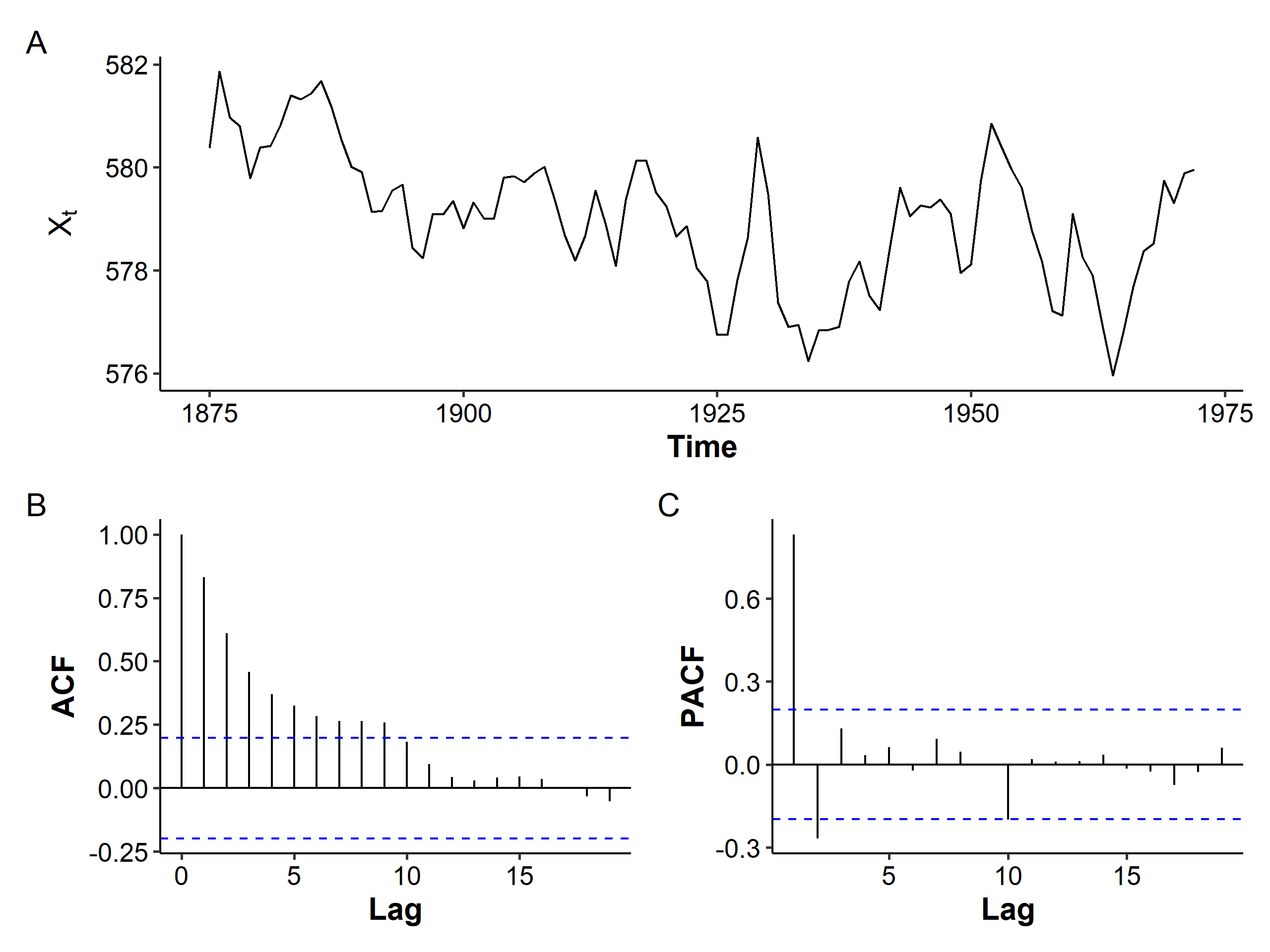
The mean seems to be decreasing over the years, and the variance seems to be slightly increasing. The ACF is more of a tail-off pattern than a slowly decreasing one. If we assume stationarity and fit an AR(2) model with an intercept:

 1
 2
 3
 4
 5
 6
 7
 8
 9
10
11
12
13

data("LakeHuron")
ar2 <- arima(LakeHuron, order = c(2, 0, 0), include.mean = T, method = "ML")
ar2

# Call:
# arima(x = LakeHuron, order = c(2, 0, 0), include.mean = T, method = "ML")

# Coefficients:
#          ar1      ar2  intercept
#       1.0436  -0.2495   579.0473
# s.e.  0.0983   0.1008     0.3319

# sigma^2 estimated as 0.4788:  log likelihood = -103.63,  aic = 215.27

Of course we could also assume nonstationarity and fit ARIMA models of different orders. So how do we choose the “best” model? In general, we should

1. minimize AIC or BIC,
2. principle of parsimony, and
3. maximize prediction ability – there’s many criteria available, such as MAPE (mean absolute percentage error).

The MAPE is given by

$$ MAPE = \frac{1}{T^} \sum_{l=1}^{T^}\left| \frac{X_{t+l} - X_t(l)}{X_{t+l}} \right| $$

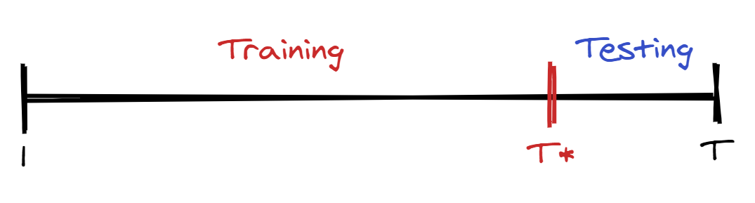
where $T^*$ is the length of the training time series. The MAPE is a measure of prediction accuracy of our forecasting model. It has a very intuitive interpretation in terms of relative error.

To calculate the MAPE, we need to split our series into two parts: one for training and one for testing. Instead of a random split as often seen in machine learning methods, we cut our series at some point and use the remaining data for testing³.

Let’s try this in R on the Lake Huron dataset. We’re going to fit four different models, starting from the AR(2) model:

 1
 2
 3
 4
 5
 6
 7
 8
 9
10
11
12
13
14
15
16
17

length(LakeHuron)
# [1] 98

lakeh <- LakeHuron[1:88]  # use a 90-10 split

ar2 <- arima(lakeh, order = c(2, 0, 0), include.mean = T, method = "ML")
ar2

# Call:
# arima(x = lakeh, order = c(2, 0, 0), include.mean = T, method = "ML")

# Coefficients:
#          ar1      ar2  intercept
#       1.0297  -0.2414   579.0638
# s.e.  0.1042   0.1070     0.3380

# sigma^2 estimated as 0.4766:  log likelihood = -92.9,  aic = 193.8

If we examine the diagnosis plots, there seems to be a spike at lag 9 for the residuals:

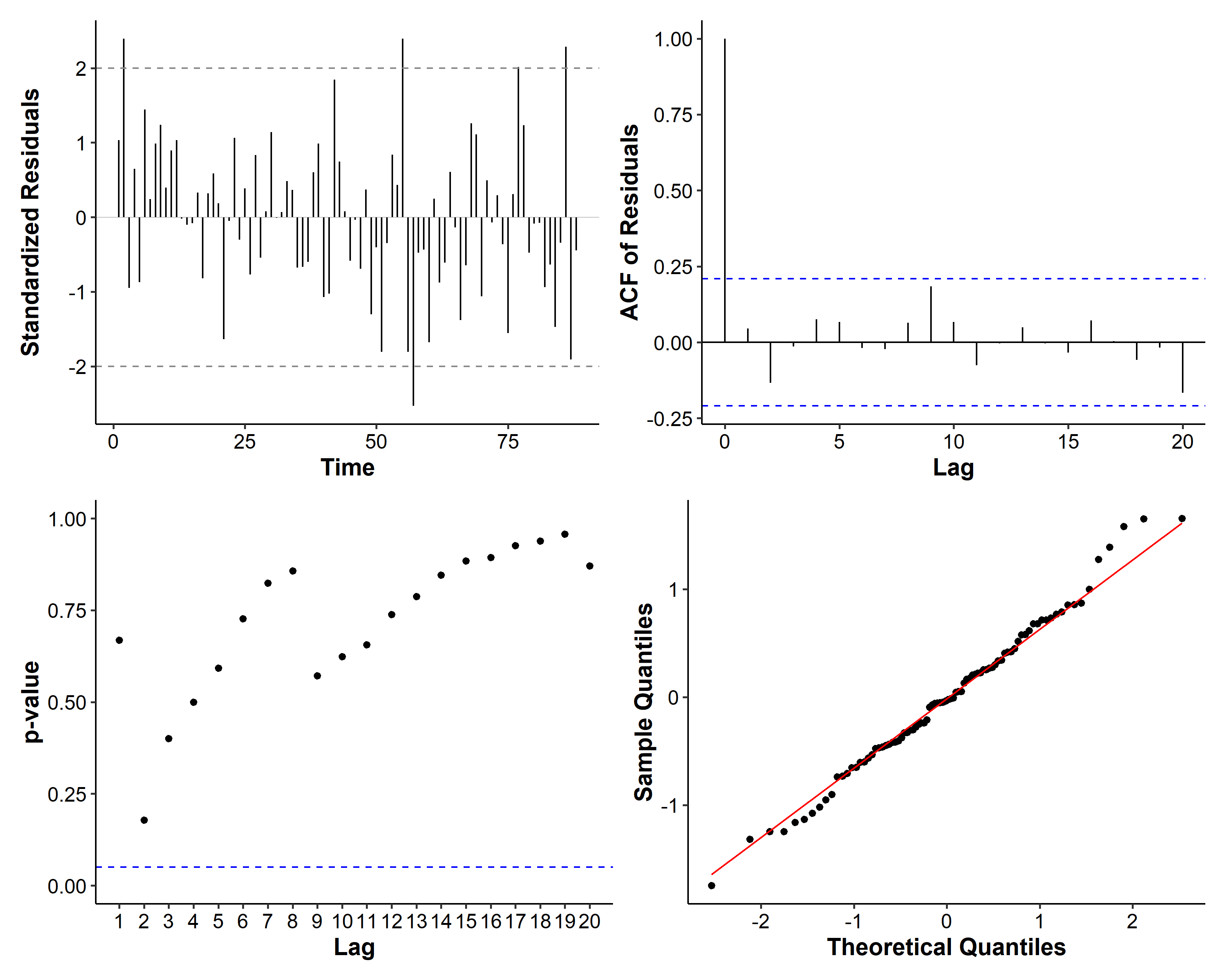
So we also consider the following models:

$$ \begin{gathered} (1 - \phi_1 B - \phi_2 B^2 - \phi_9 B^9)X_t = Z_t \\ (1 - \phi_1 B - \phi_2 B^2)X_t = (1 + \theta_9 B^9)Z_t \\ (1 - -\phi_1 B)X_t = (1 + \theta_1 B)Z_t \end{gathered} $$

where ARMA(1, 1) is considered because it’s a competing model with AR(2).

 1
 2
 3
 4
 5
 6
 7
 8
 9
10
11
12
13
14
15
16
17
18
19
20
21
22
23
24
25
26
27
28
29
30
31
32
33
34
35
36
37
38
39
40
41
42

ar9 <- arima(lakeh, order = c(9, 0, 0), include.mean = T, method = "ML",
             fixed = c(NA, NA, rep(0, 6), NA, NA))
ar9

# Call:
# arima(x = lakeh, order = c(9, 0, 0), include.mean = T, fixed = c(NA, NA, rep(0,
#     6), NA, NA), method = "ML")

# Coefficients:
#          ar1      ar2  ar3  ar4  ar5  ar6  ar7  ar8     ar9  intercept
#       0.9948  -0.2376    0    0    0    0    0    0  0.0979   579.1185
# s.e.  0.1057   0.1049    0    0    0    0    0    0  0.0661     0.4569

# sigma^2 estimated as 0.4641:  log likelihood = -91.82,  aic = 193.65

ma9 <- arima(lakeh, order = c(2, 0, 9), include.mean = T, method = "ML",
             fixed = c(NA, NA, rep(0, 8), NA, NA))
ma9

# Call:
# arima(x = lakeh, order = c(2, 0, 9), include.mean = T, fixed = c(NA, NA, rep(0,
#     8), NA, NA), method = "ML")

# Coefficients:
#          ar1      ar2  ma1  ma2  ma3  ma4  ma5  ma6  ma7  ma8     ma9  intercept
#       1.0002  -0.2248    0    0    0    0    0    0    0    0  0.2632   579.0491
# s.e.  0.1058   0.1071    0    0    0    0    0    0    0    0  0.1099     0.3835

# sigma^2 estimated as 0.4482:  log likelihood = -90.49,  aic = 190.97

arma11 <- arima(lakeh, order = c(1, 0, 1), include.mean = T, method = "ML")
arma11

# Call:
# arima(x = lakeh, order = c(1, 0, 1), include.mean = T, method = "ML")

# Coefficients:
#          ar1     ma1  intercept
#       0.7205  0.3668   579.0684
# s.e.  0.0872  0.1261     0.3452

# sigma^2 estimated as 0.4666:  log likelihood = -92,  aic = 192

Here only the NAs in the fixed parameter will be varied. We should also check the diagnosis plots for each model, but the figures are omitted for the sake of brevity. To calculate the BIC, we can use the BIC() function on the model objects. To calculate the MAPE, the following snippet can be used:

1
2

ar2.pred <- predict(ar2, 10)$pred
mean(abs((LakeHuron[89:98] - ar2.pred) / LakeHuron[89:98]))

We summarize our results in the table below. The rank of each model is given in bold for each criterion. Overall ARMA(1, 1) seems like the best model as it ranks first or second in most cases, and is a simpler model than MA(9).

After we’ve decided which model to use, we should go back and use the entire dataset including the testing data. The final model is

$$ (1 - 0.7449B)(X_t - 579.0555) = (1 + 0.3206B)Z_t, \quad \hat\sigma^2 = 0.4749 $$