Modern Nonparametric Regression
In regression, we also face the problem of underfitting / overfitting.
Here1 under-smoothing is interpolation, or connecting the dots. It gives a perfect fit to the data but is useless for anything else. Over-smoothing is ignoring $x$ altogether, and fitting $\bar{y}$ as the predicted value everywhere. It’s useless for inference. The question is can we use the data to learn about the relationship between $x$ and $y$?
We’ll focus on a single explanatory variable. The data is $(x_1, y_1)$, $(x_2, y_2)$, $\cdots$, $(x_n, y_n)$. A simple linear model
$$ y_i = \beta_0 + \beta_1x_i + \epsilon_i, \quad i=1\cdots n $$
relates $x$ and $y$ in a linear fashion. In standard parametric approaches, we assume $\epsilon_i \overset{i.i.d.}{\sim} N(0, \sigma^2)$.
We don’t want to make the normality (or any other distributional) assumption on $\epsilon_i$. We also don’t want to restrict ourselves to a linear fit, which won’t always be appropriate. The more general form is
$$ y_i = g(x_i) + \epsilon_i, \quad i = 1 \cdots n $$
Lowess
assuming $\text{median}(\epsilon_i)=0$. $g(x_i)$ is unspecified, and we want to learn this from the data. We’re being model-free and distribution-free.
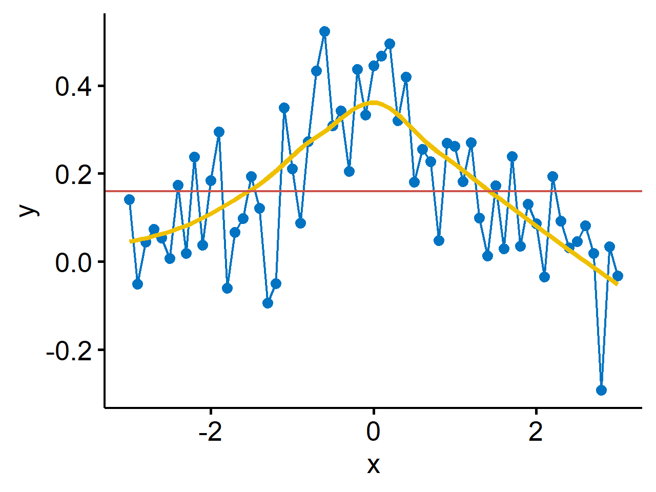
A popular method2 is called “locally weighted scatterplot smoothing” - LOWESS, or LOESS for “locally estimated scatterplot smoothing”. The basic idea if to fit a linear (or quadratic) polynomial at each data point using “weighted least squares” (does parameter estimation with different data points weighted differently), with weights that decrease as we move away from the $x_i$ at which we are fitting. Points more than a specified distance away (controlled by the span) are assigned a zero weight. The weight function is maximum at the $x_i$ value at which the fit is being made, and is symmetric about that point.
Things to consider:
- $d$: degree of polynomial to be fitted at each point (usually 1 or 2)
- $\alpha$: span, i.e. the width of the neighborhood
- $w(u)$: weight function
With these in hand, a localized (in the neighborhood), weighted least squares procedure is used to get an estimate of $g(\cdot)$ at $x_i$, call it $\hat{y}_i$. The window slides across each $x_i$, and fits a (weighted) linear ($d=1$) or quadratic ($d=2$) in each window3.
We’re looking for the general pattern, not (necessarily) local structure. This guides us in the choice of bandwidth and $d$ (less critical). Often, within a small neighborhood, functions will be roughly linear (or quadratic), so usually $d=1$ is good enough. Note that if the function is very unsmooth (lots of quick up and downs), this approach won’t work well.
Choice of neighborhood size (bandwidth / span) is a bit of trail and error as it depends on $n$. R default is $\frac{2}{3}$ of the data included in each sliding window, which will often oversmooth. As the span increases, the smoothing of the curve also increases.
For the weighting kernel (not as crucial), a popular choice is
$$
w(u) = \begin{cases} \left(1 - |u|^3\right)^3 && |u| \leq 1 \\ 0 && |u| > 1 \end{cases}
$$
This gives weights for weighted least squares. For points within the neighborhood, if the farthest points to be included in the “local” neighborhood are at a distance $\Delta$ from $x_i$, then $x_j$ (in the neighborhood) gets weight
$$ w_j = \left(1 - \left|\frac{x_j - x_i}{\Delta} \right|^3\right)^3 $$
This is done at each data point, so we get $n$ total fits. Another possibility is to robustify for the procedure by down-weighting possible outliers. In R, the lowess() function takes the following default values:
- Window of $\frac{2}{3}$ of data controlled by argument
f, the smoother span - 3 iterations of robustification controlled by argument
iter
There’s also a formula-based loess() function which is pretty similar, but has some different defaults. Note that ggplot2::geom_smooth() uses this version of LOESS.
spanis by default 0.75- degree of the polynomials $d$ is 2 by default
Penalized least squares
Recall our original problem: we had a generic model of
$$ y_i = g(x_i) + \epsilon_i $$
Suppose, in analogy to simple linear regression, we estimate $g(\cdot)$ by choosing $\hat{g}(x)$ to minimize the sum of squares
$$ \sum_{i=1}^n {\left(y_i - \hat{g}(x_i)\right)^2} $$
In the linear case, $\hat{g}(x_i)$ would be $\hat{\beta}_0 + \hat{\beta}_1 x_i$. Minimizing the sum of squares over all linear functions yields the usual least squares estimator, which is possibly an oversmooth. Minimizing over all functions yields the “connect the dots” estimator of exact interpolation, which is definitely an undersmooth.
Lowess uses the local weighting to balance between these two extremes. A different approach to getting this balance is to minimize a penalized sum of squares:
$$ \begin{equation} \label{eq:penalized-LS} U(\lambda) = \sum_{i=1}^n {(y_i - \hat{g}(x_i))^2 + \lambda J(g)} \end{equation} $$
where $\lambda$ is the tuning parameter, and $J(g)$ is the penalty function for roughness. A common choice for $J(g)$ is
$$ J(g) = \int [g’’(x)]^2dx $$
which is the integral of the squared second derivative of $g(\cdot)$ and it measures the curvature in $g$ at $x$. $\lambda$ controls the amount of smoothing - the larger it is, the more smoothing is enforced.
Cubic spline
We want “optimal” solution to Equation $\eqref{eq:penalized-LS}$. Let $\eta_1 < \eta_2 < \cdots < \eta_k$ be a set of ordered points, or knots, contained in some interval $(a, b)$. A cubic spline is defined as a continuous function $r$ such that
- $r$ is a cubic polynomial over each $(\eta_1, \eta_2)$, $(\eta_2, \eta_3)$, $\cdots$
- $r$ has continuous first and second derivatives at the knots, which ensures smoothness of the curves at the knots.
In general, an $M^{th}$-order spline is a piecewise $M-1$ degree polynomial with $M-2$ continuous derivatives at the knots. The simplest spline has degree 0 and is a step function. A spline with degree 1 is called a linear spline.
A spline that is linear beyond the boundary knots ($\eta_1$ and $\eta_k$) is called a natural spline. In mathematical terms, the second derivatives of the spline polynomials are set to 0 and the endpoints of the interval $(a, b)$.
The cubic spline ($M=4$) are the most commonly used and solve our penalized problem4. No discontinuities (or jumps) at the knots means that the functions connect smoothly, and edge effects beyond $\eta_1$ and $\eta_k$ are handled through the linear fit. The function $\hat{g}(x)$ that minimizes $U(\lambda)$ with penalty $\int[g’’(x)]^2$ is a natural cubic spline with knots at the data points. Our estimator $\hat{g}(x)$ is called a smoothing spline.
What does $\hat{g}(x)$ look like? We can construct a basis for a set of splines:
$$ \begin{gather*} h_1(x) = 1 \\ h_2(x) = x \\ h_3(x) = x^2 \\ h_4(x) = x^3 \\ \vdots \\ h_j(x) = (x - \eta_{j-4})^3_+, \quad j = 5, \cdots, k+4 \end{gather*} $$
where $(x - \eta_{j-4})^3_+ = 0$ if $(x - \eta_{j-4})^3 < 0$. The set ${h_1, h_2, \cdots, h_{k+4}}$ is a basis for the set of cubic splines at these knots, called the truncated power basis. This means any cubic spline $g(x)$ with these same knots can be written as
$$ g(x) = \sum_{j=1}^{k+4} {\beta_j h_j(x)} $$
where $h_j(x)$ is known, and we just need to estimate $\beta_j$ e.g. by least squares. There are also other sets of basis functions.
In R, there’s a library splines.
smoothing.splines()places knots at each data point and performs smoothing splines.ns()is for general natural splines, and we need to specify the number and locations of knots, which is not an easy question to answer!bs()generates a basis function set for splines which we can then use for other things. This also requires specifying the number and locations of knots.
Remarks
- $\lambda$, the tuning parameter, controls the roughness of the fit, so it also somewhat shrinks the basis functions.
- We need to be aware of and account for edge effects. The fit isn’t going to look as good at the ends.
- $\lambda$ controls the bias-variance tradeoff in the spline setting.
- $\lambda = 0 \Rightarrow$ no effect of the penalty term $\Rightarrow$ exact interpolation $\Rightarrow$ low bias, high variance.
- $\lambda \rightarrow \infty \Rightarrow$ perfectly smooth (linear) fit $\Rightarrow$ a line that passes as close to the data as possible $\Rightarrow$ high bias, low variance.
- Intermediate values of $\lambda$ balance the two, and we get a reasonably smooth function that passes near the data.
R code for generating the figure:
↩︎1 2 3 4 5 6 7 8 9 10 11library(tidyverse) library(ggpubr) set.seed(42) df <- tibble( x = seq(-3, 3, by = 0.1), y = dnorm(x, 0, 1) + rnorm(length(x), 0, 0.1) ) ggline(df, x = "x", y = "y", color = "#0073C2", numeric.x.axis = T)+ geom_smooth(color = "#EFC000", method = "loess", se = F)+ geom_abline(slope = 0, intercept = mean(df$y), color = "#CD534C")Cleveland, William S. “Robust locally weighted regression and smoothing scatterplots.” Journal of the American statistical association 74.368 (1979): 829-836. ↩︎
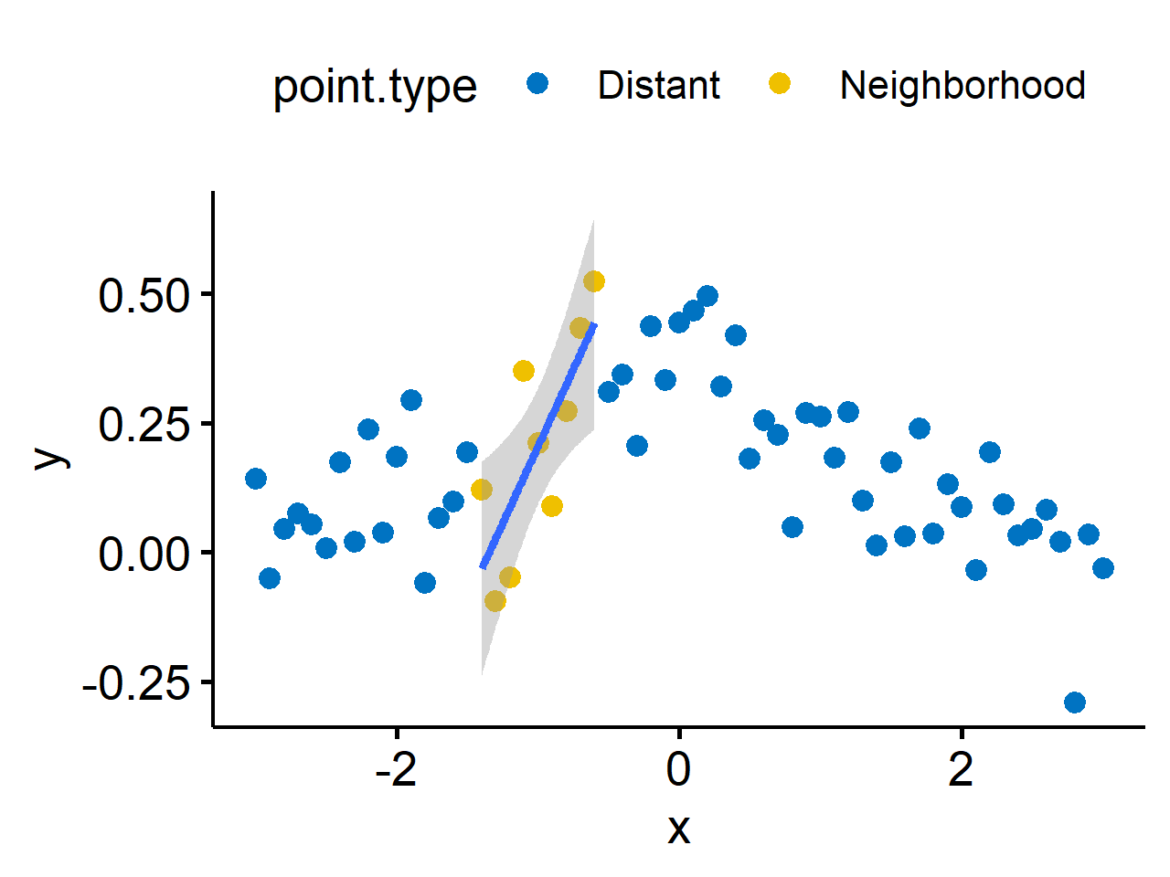
R code for plotting:
↩︎1 2 3 4 5 6 7 8 9 10 11library(tidyverse) library(ggpubr) set.seed(42) df <- tibble( x = seq(-3, 3, by = 0.1), y = dnorm(x, 0, 1) + rnorm(length(x), 0, 0.1), point.type = ifelse(x > -1.5 & x < -0.5, "Neighborhood", "Distant") ) ggscatter(df, "x", "y", color = "point.type", palette = "jco") + geom_smooth(data = subset(df, x > -1.5 & x < -0.5), method = "lm")
| May 06 | Density Estimation | 6 min read |
| May 06 | Bootstrap | 11 min read |
| May 06 | Categorical Data | 17 min read |
| May 05 | Correlation and Concordance | 9 min read |
| May 04 | Basic Tests for Three or More Samples | 10 min read |