Basic Tests for Three or More Samples
The following methods discussed are nonparametric analogues to analysis of variance (ANOVA). When the ANOVA assumptions (normality and homogeneity of variances in residuals) cannot be met, a nonparametric test is appropriate.
Notations
Suppose we have independent random samples (independence within and across samples). The $i^{th}$ sample has $n_i$ observations, $i = 1, \cdots, k$. The general question would be equality of means / medians, or identical distributions.
- $x_{ij}$ - observations from sample $i$ where $j = 1, \cdots, n_i$
- $N = \sum\limits_{i=1}^k{n_i}$ - total number of observations across all samples
- $r_{ij}$ - rank of $x_{ij}$ in the combined sample (ranges from $1$ to $N$)
- $S_i = \sum\limits_{j=1}^{n_i}{r_{ij}}$ - sum of ranks of observations in the $i^{th}$ sample (group)
The Kruskal-Wallis test
The K-W test extends the WMW test via the Wilcoxon formulation. It can be used as an overall test for equality of means / medians at the population level, when samples are from otherwise identical continuous distributions (i.e. shifts of location).
It can also be used as a test for equality of distribution against an alternative that at least one of the populations tends to yield larger observations than at least one of the other populations.
Under $H_0$ (equality of means / medians), all of the $S_i$ should be “roughly similar” because each sample will have small, medium and large ranks. Under $H_1$ (not all the same), some $S_i$ should be “larger” than others, and some “smaller”. We’d have clusters of small / large ranks in some of the samples. The test statistic
$$ T = \frac{12S_k}{N(N+1)} - 3(N+1) \quad \text{where } S_k = \sum\limits_{i=1}^k{\frac{S_i^2}{n_i}} $$
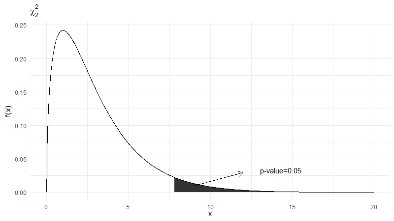
$S_k$ will be inflated if there’s a cluster of large ranks in one or two of the samples. A large $T$ is evidence against $H_0$, as shown in the figure below1. If $N$ is moderate or large, then under $H_0$, $T \dot\sim \chi^2_{(k-1)}$.
In R, the function kruskal.test() can be used in two ways:
- Input a data vector
xand a vector of group indicatorsg(xandgshould both have length $N$). Now we can callkruskal.test(x, g). This method emphasizes the Wilcoxon nature. - Use the same input, but use a formula
kruskal.test(x ~ g). This model formulation emphasizes the connection to ANOVA.
A very useful R package coin includes more functionality for this test.
Multiple comparisons
If $H_0$ is rejected, i.e. there’s a difference among the $k$ groups, we may be interested in exploring which groups differ. This is the multiple comparisons problem. There are a lot of different ways to address this issue, and we’ll look at one of these - consider all $\binom{k}{2}$ pairwise comparisons. For each pair of samples $i$ and $j$:
$$ \left|\frac{S_i}{n_i} - \frac{S_j}{n_j}\right| > t_{1 - \frac{\alpha}{2}} \left[\frac{N(N+1)}{12} - \frac{(N_1-T)}{N-k}\right]^{\frac{1}{2}}\left(\frac{1}{n_i} + \frac{1}{n_j}\right)^{\frac{1}{2}} $$
where the LHS is the average rank for observations in sample $i$ ($j$), and the RHS is a measure of variability in the differences. The $t_{1 - \frac{\alpha}{2}}$ is the $1 - \frac{\alpha}{2}$ upper quantile from the $t$-distribution with $N - k$ degrees of freedom.
The problem now is, what is the “right” $\alpha$ to use here? A naïve approach is to test all $\binom{k}{2}$ post-hoc (after rejecting $H_0$ of overall equality of means/medians) at the same level $\alpha$, say $0.05$. The problem with the approach is that our Type I error probability is inflated above $0.05$. The more comparisons there are, the more inflation there is, which makes our inference unreliable.
We need to make an adjustment. There’s also lots of ways to do this! One popular way to adjust this is the Bonferroni correction. The idea is to control the overall Type I error probability at level $\alpha$ by testing each of the post-hoc comparisons at level $\frac{\alpha}{\binom{k}{2}}$ instead of at level $\alpha$. With a more stringent cutoff, we make it harder to reject a null hypothesis of “no difference”.
Ties in the data
We use the mid-ranks for ties as before. Define:
$$ \begin{gather*} S_r = \sum_{i,j}{r_{ij}^2} \\ C = \frac{1}{4}N(N+1)^2 \end{gather*} $$
and our test statistic:
$$ T = \frac{(N-1)(S_k - C)}{S_r - C} $$
If there are no ties, this reduces to the previous statistic. This will be approximately $\chi^2_{(k-1)}$ for large $N$.
The Jonckheere-Terpstra test
The J-T test is a test for a directional alternative. This is more specific than the previous K-W test as now there’s a priori ordering, i.e. $H_1$: $\theta_1 \leq \theta_2 \leq \cdots \leq \theta_k$ with at least one strict inequality. Here we have ordered means/medians. This test has more statistical power than the K-W test. The K-W can still be used, but we’ll get a more sensitive analysis if we use a test that is more specific for this type of alternative.
Importantly, as with all cases of ordered alternatives, the order of the groups and the direction of the alternative need to be set prior to data collection based on theory, prior experience, etc. You can’t look at the data and then decide on order, or decide to do an ordered alternative. The J-T test is designed for this case, and extends the Mann-Whitney two-sample formulation. As usual, this is best explained in an example!
Braking distance taken by motorists to stop when driving at various speeds. A prior (before seeing any data) is that braking distance increases as driving speed increases. A subset of the data is given in the following table.
| Sample | Speed (mph) | Braking distances (feet) |
|---|---|---|
| 1 | 20 | 48 |
| 2 | 25 | 33, 48, 56, 59 |
| 3 | 30 | 60, 67, 101 |
| 4 | 35 | 85, 107 |
The speeds are ordered in the data. We expect braking distance to increase. Our procedure is with $k$ samples (here $k=4$), compute all pairwise M-W test statistics. Add all of these up, i.e. compute all of $U_r$s relevant to the $r^{th}$ sample ($r = 1, \cdots, k-1$) and any sample $s$ for which $s > r$. In example, $U = U_{12} + U_{13} + U_{14} + U_{23} + U_{24} + U_{34}$, e.g. $U_{12} =$ number of sample $2$ values that exceed each sample $1$ value $= 2.5$ ($48$ counts as a half since it’s equal to the value in sample $1$). Likewise: $U_{13} = 3, U_{14} = 2, U_{23} = 12, U_{24} = 8, U_{34} = 5$. In total, our test statistic $U = 32.5$.
We could potentially do an exact calculation by looking at all the possible configurations. Or we could use simulation where we randomly sample from all possible configurations. The final way is using asymptotic approximation.
In R, the package clinfun has a function called jonckheere.test() that does the job for us. When $N < 100$ and there are no ties, it does an exact calculation. Otherwise, a normal approximation is used:
$$ \begin{gather*} E(U) = \frac{1}{4}\left(N^2 - \sum\limits_{i=1}^k{n_i^2}\right) \\ Var(U) = \frac{1}{72}\left[N^2(2N+3) - \sum\limits_{i=1}^k{\left[n_i^2(2n_i+3)\right]}\right] \end{gather*} $$
In our case, since we have an ordered alternative, an one-sided test should be used. Also, since we have very small samples, can we trust a normal approximation?
If we had perfect separation (i.e. all observations in sample $1$ < all observations in sample $2$ < $\cdots$ without overlap), then the value of the test statistic $U$ would be $35$. Our observed value is pretty close to that. We have circumstantial evidence against $H_0$. But the question is, how many configurations do we have in total? How many of them have value of $U > 32.5$?
The exact calculation (ignores ties) gives a p-value of 0.0011. The normal approximation (we have small samples) gives a p-value of 0.0022. Both values are very small, and we have converging evidence against $H_0$. We may conclude that braking distance increases as driving speed increases.
The median test
Another easy generalization is the median test. We have $k$ independent samples instead of two:
$$ \begin{gather*} H_0: \theta_1 = \theta_2 = \cdots = \theta_k \\ H_1: \text{not all } \theta_i \text{ are equal} \end{gather*} $$
We can get a $K \times 2$ contingency table following the same procedure as in two independent samples.
| sample 1 | sample 2 | $\cdots$ | sample k | ||
|---|---|---|---|---|---|
| Above M | A | ||||
| Below M | B | ||||
| $n_1$ | $n_2$ | $\cdots$ | $n_k$ | $N$ |
Column margins $n_1, \cdots, n_k$ are fixed by design, and row margins $A$ and $B$ are constrained by use of median ($A \approx B$). What doesn’t translate from the $2 \times 2$ table is - what does a “more extreme” table mean now? Another thing is just knowing one cell value isn’t enough to fill out the whole table since we have more degrees of freedom here. We need $k-1$ of them.
Because of those issues, we’ll just go straight to an approximation here. Our test statistic
$$ T = \sum\limits_{i=1}^k {\frac{\left(a_i - \frac{n_i A}{N}\right)^2}{\frac{n_i A}{N}}} + \sum\limits_{i=1}^k{\frac{\left(b_i - \frac{n_i B}{N}\right)^2}{\frac{n_i B}{N}}} $$
where $\frac{n_iA}{N}$ is the expected number of cases above $M$ for group $i$ under $H_0$. This test statistic is essentially the $\chi^2$ test for independence, which we’ll talk about more in later chapters.
$$ \chi^2 = \sum_{i=1}^m{\frac{(O_i - E_i)^2}{E_i}} $$
The Friedman test
The Friedman test makes inference for several related samples. Its parametric analogy is the two-way classification ANOVA from a randomized block design2.
Data: the data we have are $b$ independent “blocks” (patients, plots of land, etc.) and $t$ “treatments” which are applied to (or measured on) each block. So the data are a $b \times t$ array, as usually we put blocks along the rows and treatments along the columns. Blocks are independent; measurements are dependent within a block.
Procedure: within each block, independently rank the observations from $1$ (smallest) to $t$ (largest). The null hypothesis: all treatments have the same effect; the alternative is not $H_0$. The test statistic: $$ T = \frac{12}{bt(t+1)} \sum\limits_{i=1}^t {S_i^2} - 3b(t+1) $$
where $S_i$ is the sum over all blocks of the ranks allocated to treatment $i$ (rank along the rows, sum across the columns). The sum part is the core of the test statistic that encapsulates the procedure, and the other constants are derived from mathematical theories that help form a distribution we can work with later.
For $b, t$ that are “not too small”, $T$ is approximately $\chi^2_{(t-1)}$ under $H_0$. The test is to look at whether we fall in the far right tail of the $\chi^2$ distribution. Again, it’s much easier to explain the test with an example.
Example: 7 students’ pulse rate per min. was measured (i) before exercise, (ii) immediately after exercise, and (iii) 5 minutes after exercise. Our $H_0$ is there’s no effect of exercise / rest on pulse rates, and the alternative is not $H_0$.
Results (repeated measures):
| Student | Before | Right after | 5min. after |
|---|---|---|---|
| 1 | 72 | 120 | 76 |
| 2 | 96 | 120 | 95 |
| 3 | 88 | 132 | 104 |
| 4 | 92 | 120 | 96 |
| 5 | 74 | 101 | 84 |
| 6 | 76 | 96 | 72 |
| 7 | 82 | 112 | 76 |
Our procedure says rank along each row separately:
| Student | Before | Right after | 5min. after |
|---|---|---|---|
| 1 | 1 | 3 | 2 |
| 2 | 2 | 3 | 1 |
| 3 | 1 | 3 | 2 |
| 4 | 1 | 3 | 2 |
| 5 | 1 | 3 | 2 |
| 6 | 2 | 3 | 1 |
| 7 | 2 | 3 | 1 |
then sum ranks along each column, which gives
$$ S_1 = 10, S_2 = 21, S_3 = 11 $$
In data, $T = 10.57$. Compare to $\chi^2_{(2)}$ at $\alpha = 0.05$, where $T_\alpha = 5.99$. We have strong evidence against $H_0$.
So far we’ve focused on location and distribution inferences. What about association analyses?
R code used for generating this figure inspired by this post. See
?plotmathfor symbol details↩︎1 2 3 4 5 6 7 8 9 10 11 12 13 14 15 16 17 18 19 20 21 22 23library(tidyverse) df <- tibble( x = seq(0, 20, 0.01), y = dchisq(x, 3) ) rejection.region <- df %>% filter(x >= qchisq(0.95, 3)) %>% bind_rows(tibble( x = qchisq(0.95, 3), y = 0 )) ggplot(rejection.region, aes(x, y))+ geom_polygon(show.legend = F)+ geom_line(data = df, aes(x, y))+ annotate("segment", x = 9, y = 0.01, xend = 12, yend = 0.03, arrow = arrow(length = unit(0.3, "cm")))+ annotate("text", label="p-value=0.05", x=14.3, y=0.033, size=4)+ xlab(expression(x))+ ylab(expression(f(x)))+ ggtitle(expression(chi[2]^2))+ theme_minimal()According to Wikipedia, The Friedman test is similar to the repeated measures ANOVA. ↩︎
| May 08 | Modern Nonparametric Regression | 8 min read |
| May 06 | Density Estimation | 6 min read |
| May 06 | Bootstrap | 11 min read |
| May 06 | Categorical Data | 17 min read |
| May 05 | Correlation and Concordance | 9 min read |