Other Single Sample Inferences
Previously we talked a lot about location inference, which is looking at the mean or median of the population distribution, or in fancier words, inferences about centrality. In this chapter we explore whether our sample is consistent with being a random sample from a specified (continuous) distribution at the population level.
Under $H_0$, the population distribution is completely specified with all the relevant parameters, such as a normal distribution with given mean and variance, or a uniform distribution with given lower and upper limits, or at least it’s some specific family of distributions.
Kolmogorov’s test
The Kolmogorov's test is a widely used procedure. The idea is to look at the empirical CDF $S_n(x)$, which is a step function that has jumps of $\frac{1}{n}$ at the observed data points.
We mentioned before that as $n \rightarrow \infty$, it becomes “close” to the true CDF, $F(x) = P(X \leq x)$. So, $S_n(x)$ is a consistent estimator for $F(x)$.
If our data really are a random sample from the distribution $F(x)$, we should then be seeing evidence of that in $S_n(x) - F(x)$ and $S_n(x)$ should be “close”. Under $H_0$, $F(x)$ is completely specified, so it’s known. $S_n(x)$ is determined by the data, so it’s known as well, which means we can compare them explicitly!
The logic of the test statistic is if $x_1, x_2, \cdots, x_n$ are a sample from a population with distribution $F(x)$, then the maximum difference between the CDF under $H_0$ and the empirical CDF should be small. The larger the maximum difference is, the more evidence against $H_0$. It’s generally a good idea to plot the empirical CDF together with the hypothesized to see visually how close they are1:
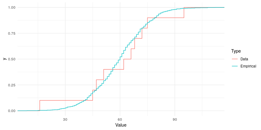
Our Test statistic is the maximum vertical distance between $F(x)$ and $S_n(x)$, or
$$ T = \sup_x \left|F(x) - S_n(x) \right| $$
for a two-sided test for a two-tailed alternative. Deriving the exact distribution in this case is much more complex. In R, the function ks.test() does the job. You have to specify what distribution to compare to, e.g. ks.test(dat, "pnorm", 2, 4) to test whether dat look like a sample from $N(2, 4)$.
More typically, though, we won’t know the values of the parameters that define the distribution. In other words, we have unknown parameters that need to be estimated. If we use the Kolmogorov test with estimated values (from the sample) of the parameters, the distribution of the test statistic $T$ changes.
Lilliefors test for normality
The Lilliefors test is a simple modification of Kolmogorov’s test. We have a sample $x_1, x_2, \cdots, x_n$ from some unknown distribution $F(x)$. Compute the sample mean and sample standard deviation as estimates of $\mu$ and $\sigma$, respectively:
$$ \begin{gather*} \bar{x} = \frac{1}{n}\sum\limits_{i=1}^n x_i \\ S = \sqrt{\frac{1}{n-1} \sum\limits_{i=1}^n (x_i - \bar{x})^2} \end{gather*} $$
Use these to compute “standardized” or “normalized” versions of the data to test for normality:
$$ \begin{aligned}Z_i = \frac{x_i - \bar{x}}{S} && i = 1, 2, \cdots, n\end{aligned} $$
Compare the empirical CDF of the $Z_i$ to the CDF of $N(0, 1)$, as with the Kolmogorov procedure. Alternatively, use the original data and compare to $N(\bar{x}, S^2)$. Here $H_0$: random sample comes from a population with the normal distribution with unknown mean and standard deviation, and $H_1$: the population distribution is non-normal.
This is a composite test of normality (testing multiple things simultaneously). We can obtain the distribution of the test statistics via simulation. In R, we can use the function nortest::lillie.test().
Remarks
We computed $\bar{x}$ and $S$ and used those as estimators for the normal mean and s.d. in the population. Basically follow the Kolmogorov procedure with $\bar{x}$ and $s$.
Lilliefors vs. Kolmogorov - procedurally very similar, but the reference distribution for the test statistic changes because we estimate the population mean and standard deviation.
Lilliefors found this reference distribution by simulation in the late 1960s2. The idea was to generate random normal variates. For various values of sample size $n$, these random numbers are grouped into “samples”. For example, if $n = 8$, a simulated sample of size 8 from $N(0, 1)$ (under $H_0$) is generated. The $Z_i$ values are computed as described earlier. The empirical CDF is compared to the $N(0, 1)$ CDF, and the maximum vertical discrepancy is found / recorded. Repeat this thousands of times to build up the simulated reference distribution for the test statistic under $H_0$ when $n=8$. Repeat for many different sample sizes. As the number of simulations increases for a given sample size, the approximation improves.
Test for the exponential
Let’s look at a different example, the exponential. Our $H_0$: random sample comes from the exponential distribution
$$ F(x) = \begin{cases} 1 - e^{-\frac{x}{\theta}}, & x \geq 0 \\ 0, & x < 0 \end{cases} $$
where $\theta$ is an unknown parameter, vs. $H_1$: distribution is not exponential. Another composite null. We can compute
$$ Z_i = \frac{x_i}{\bar{x}} $$
where we use $\bar{x}$ to estimate $\theta$. Consider the empirical CDF of $Z_1, Z_2, \cdots, Z_n$. Compare it to
$$ F(x) = 1 - e^{-x} $$
and find the maximum vertical distance between the two. This is the test statistic for the Lilliefors test for exponentiality. Tables for the exact distribution for this case exist, but not in general. The R package KScorrect tests against many hypothesized distributions.
Another Test for Normality
The Shapiro-Wilk test is another important test for normality which is used quite often in practice. We again have a random sample $x_1, x_2, \cdots, x_n$ with unknown distribution $F(x)$. $H_0$: $F(x)$ is a normal distribution with unspecified mean and variance, vs. $H_1$: $F(x)$ is non-normal.
The idea essentially is to look at the correlation between the ordered sample values (order statistics from the sample) and the expected order statistics from $N(0, 1)$. If the null holds, we’d expect this correlation to be near 1. Smaller values are evidence against $H_0$. A Q-Q plot has the same logic as this test.
For the test more specifically:
$$ W = \frac{1}{D} \left[ \sum\limits_{i=1}^k a_i \left( x_{(n - i + 1)} - x_{(i)} \right) \right]^2 $$
- $k = \frac{2}{n}$ if $n$ is even, otherwise $k = \frac{n-1}{2}$
- $x_{(j)}$ are the order statistics for the sample
- $a_j$ are the expected order statistics from $N(0, 1)$, obtained from tables
- $D = \sum\limits_{i=1}^n (x_i - \bar{x})^2$
We may also see it written as
$$ W =\frac {\left[ \sum\limits_{i=1}^n a_i x_{(i)} \right]^2}{D} $$
With large samples, the chance to reject $H_0$ increases - even small departures from normality will be detected, and formally lead to rejecting $H_0$ even if the data are “normal enough”. Many parametric tests (such as the t-test) are pretty robust to departures from normality.
The takeaway here is to always think about what you’re doing. Don’t apply tests blindly - think about results, what they really mean, and how you will use them.
Runs or Trends
The motivation here is that many basic analyses make the assumption of a random sample, i.e. independent, identically distributed observations (i.i.d). When this assumption doesn’t hold, we need a different analysis strategy (e.g. time series, spatial statistics, etc.) depending on the characteristics of the data.
Cox-Stuart test
When the data are taken over time (ordered in time), there may be a trend in the observations. Cox and Stuart3 proposed a simple test for a monotonically increasing or decreasing trend in the data. Note that monotonic doesn’t mean linear, but simply a consistent tendency for values to increase or decrease.
The procedure is based on the sign test. Consider a sample of independent observations $x_1, x_2, \cdots, x_n$. If $n = 2m$, take the differences
$$ x_{m+1} - x_1, x_{m+2} - x_2, \cdots, x_{2m} - x_m $$
If $n = 2m + 1$, omit the middle value $x_{m+1}$ and calculate $x_{m+2} - x_1, \cdots$.
If there is an increasing trend over time, we’d expect the observations earlier in the series will tend to be smaller, so the differences will tend to be positive, and vice versa if there is an decreasing trend. If there’s no monotonic trend, the observations differ by random fluctuations about the center, and the differences are equally likely to be positive or negative.
Under $H_0$ of no monotonic trend, the $+/-$ signs of the differences are $Bin(m, 0.5)$. That’s a sign test scenario!
Example: The U.S. Department of Commerce publishes estimates obtained for independent samples each year of the mean annual mileages covered by various classes of vehicles in the U.S. The figures for cars and trucks (in $1000$s of miles) for the years $1970-1983$ are:
| Cars | 9.8 | 9.9 | 10.0 | 9.8 | 9.2 | 9.4 | 9.5 |
|---|---|---|---|---|---|---|---|
| 9.6 | 9.8 | 9.3 | 8.9 | 8.7 | 9.2 | 9.3 | |
| Trucks | 11.5 | 11.5 | 12.2 | 11.5 | 10.9 | 10.6 | 11.1 |
| 11.1 | 11.0 | 10.8 | 11.4 | 12.3 | 11.2 | 11.2 |
Is there evidence of a monotonic trend in each case?
$$ \begin{aligned} &H_0: \text{no monotonic trend} \\ \text{vs. } &H_1: \text{monotonic trend} \end{aligned} $$
We don’t specify increasing or decreasing because we don’t have that information, so it’s a two-sided alternative.
For cars, all the differences are negative. When $X \sim Bin(7, 0.5)$, $P(X = 7) = 0.5^7 = 0.0078125$. We have a two-sided alternative, so we need to consider also $X=0$, which by symmetry has the same probability, so we get a p-value $\approx 0.0156$. This is reasonably strong evidence against $H_0$.
For trucks, we have 4 negative differences and 3 positive differences, which is supportive of $H_0$, in fact, the most supportive you could be with just 7 differences.
Runs test
Note that the sign test does not account for, or “recognize”, the pattern in the signs for the trucks. There is evidence for some sort of trend, but since it’s not monotonic, the sign test can’t catch it. It also can’t find periodic, cyclic, and seasonal trends, because it only counts the number of successes / failures. We need a different type of procedure.
One possibility is the runs test, which looks for patterns in the successes / failures. We’re looking for patterns that may indicate a “lack of randomness” in the data. Suppose we toss a coin 10 times and see
$$ \text{H, T, H, T, H, T, H, T, H, T} $$
We’d suspect non-randomness because of the constant switching back and forth. Similarly, if we saw $$ \text{H, H, H, T, T, T, T, H, H, H} $$
We’d suspect non-randomness because of too few switches, or too “blocky”.
For tests of randomness, both the numbers and lengths of runs are relevant. In the first case we have 10 runs of length 1 each, and in the second case we have 3 runs - one of length 3, followed by one of length 4, and another of length 3. Too many runs and too few are both indications of lack of randomness. Let
$$ \begin{aligned} &r\text{: the number of runs in the sequence} \\ &N \text{: the length of the sequence} \\ &m \text{: the number of observations of type 1 (e.g. H)} \\ &n = N - m \text{: the observations of type 2} \end{aligned} $$
Our hypotheses are $$ \begin{aligned} &H_0: \text{independence / randomness} \\ \text{vs. } &H_1: \text{not }H_0 \end{aligned} $$
We reject $H_0$ if $r$ is too big or too small. To get a handle on this, we need to think about the distribution of the number of runs for a given sequence length. We’d like to know
$$ P(R = r) = \frac{\text{# of ways of getting r runs}}{\text{total # of ways of arranging H/Ts}} $$
This is conceptually easy, but doing this directly would be tedious for a even moderate $N$. We can use combinatorics to work it out. The denominator is the number of ways to pick $m$ out of $N$: $\binom{N}{m}$. As for the numerator, we need to think about all the ways to arrange $m$ Hs and $n$ Ts to get $r$ runs in total:
$$ \begin{gather*} P(R = 2s + 1) = \frac{\binom{m-1}{s-1} \binom{n-1}{s} + \binom{m-1}{s} \binom{n-1}{s-1}}{\binom{N}{m}} \\ P(R = 2s) = \frac{2 \cdot \binom{m-1}{s-1} \binom{n-1}{s-1} }{\binom{N}{m}} \end{gather*} $$
In principle, we can use these formulas to compute tail probabilities of events, and hence p-values, if $m$ and $n$ aren’t too large (both $\leq 20$). We could run into numerical issues if this isn’t the case, and computing the tail probabilities is tedious, so we also have a normal approximation:
$$ \begin{gather*} E(R) = 1 + \frac{2mn}{N} \\ Var(R) = \frac{2mn(2mn - N)}{N^2(N-1)} \end{gather*} $$
Asymptotically,
$$ Z = \frac{R - E(R)}{\sqrt{Var(R)}} \dot\sim N(0, 1) $$
We can still improve by continuity correction: add $\frac{1}{2}$ to numerator if $R < E(R)$ and substract $\frac{1}{2}$ if $R > E(R)$.
The question of interest overall is randomness, or lack of randomness, thereof the test is two-sided by nature. There are two extremes of run behavior:
- clustering or clumping of types - small number of long runs is evidence (one-sided).
- alternating pattern of types - large number of runs is evidence of an alternating pattern (again, in an one-sided perspective).
Runs test for multiple categories
We may also take a simulation-based approach. The goal is to find critical values, or p-values empirically based on simulation, rather than using the normal approximation.
The procedure is to generate a large number of random sequences of length $N$, with $m$ of type 1 events and $n$ of type 2 events (e.g. use R to generate a random sequence of 0’s and 1’s, the probabilities for $m$ and $n$ comes from the original data - essentially permuting the original sequence). Count the number of runs in each sequence, and this number is what we found for our test statistic based on the data. The generated data is what we expect if the null is reasonable. Gathering all of these together gives an empirical distribution for the number of runs you might expect to see in a sequence of length $N$ ($m$ of type 1, $n$ of type 2) if $H_0$ is reasonable.
If $N$ (hence also $m, n$) is small, we can compute the exact probabilities. Also, if $N$ is small or moderate, if you generate a lot of random sequences, you will see a lot of repeated sequences.
What if we have more than 2 types of events? Smeeton and Cox4 described a method for estimating the distribution of the number of runs by simulating permutations of the sequence of categories. Suppose we have $k$ different outcomes / events, and let $n_i$ denote an observation of type $i$. We have $N = \sum\limits_{i=1}^k n_i$ - the total length of the sequence, and $p_i = \frac{n_i}{N}$ - proportion of observation of type $i$.
We can again use the simulation approach here: generate a lot of sequences of length $N$, with $n_1$ of type 1, $n_2$ of type 2, …, $n_k$ of type $k$, and count the number of runs in each sequence.
p-values: suppose we have $1000$ random sequences of length $N$, and the number of runs ranges from $5$ to $25$. In the $1000$ simulations, we need to take down how many showed $5$ runs, $6$ runs, …, $25$ runs. If we observed $12$ runs in our data, the tail probability is $P(R \leq 12)$, and find the tail probability on the other tail by symmetry (e.g. $(5, 6, 24, 25)$).
Normal approximation: Schuster and Gu5 proposed an asymptotic test based on the normal distribution makes use of the mean and variance of the number of runs: $$ \begin{gather*} E(R) = N \left( 1 - \sum\limits_{i=1}^k {p_i^2}\right) + 1 \\ Var(R) = N \left[ \sum\limits_{i=1}^k {\left(p_i^2 - 2p_i^3 \right)} + \left(\sum\limits_{i=1}^k {p_i^2} \right)^2\right] \end{gather*} $$
Use these in a normal approximation:
$$ Z = \frac{R - E(R)}{\sqrt{Var(R)}} \dot\sim N(0, 1) $$
where $R$ denotes the observations in our sample. Barton and David6 suggest that the normal approximation is adequate for $N > 12$, no matter what the number of categories is.
So far we’ve been talking about inferences on single samples. Next we’ll take a step further and discuss paired samples.
Below is the R code for generating the plot:
↩︎1 2 3 4 5 6 7 8 9 10 11 12library(tidyverse) set.seed(42) tibble( Type = c(rep("Empirical", 1000), rep("Data", 10)), Value = c( round(rnorm(1000, mean=60, sd=15)), round(rnorm(10, mean = 60, sd = 15)) ) ) %>% ggplot(aes(Value, color = Type)) + stat_ecdf(geom = "step")+ theme_minimal()Lilliefors, H. W. (1967). On the Kolmogorov-Smirnov test for normality with mean and variance unknown. Journal of the American statistical Association, 62(318), 399-402. ↩︎
Cox, D. R., & Stuart, A. (1955). Some quick sign tests for trend in location and dispersion. Biometrika, 42(1/2), 80-95. ↩︎
Smeeton, N., & Cox, N. J. (2003). Do-it-yourself shuffling and the number of runs under randomness. The Stata Journal, 3(3), 270-277. ↩︎
Schuster, E. F., & Xiangjun, G. (1997). On the conditional and unconditional distributions of the number of runs in a sample from a multisymbol alphabet. Communications in Statistics-Simulation and Computation, 26(2), 423-442. ↩︎
Barton, D. E., & David, F. N. (1957). Multiple runs. Biometrika, 44(1/2), 168-178. ↩︎
| May 08 | Modern Nonparametric Regression | 8 min read |
| May 06 | Density Estimation | 6 min read |
| May 06 | Categorical Data | 17 min read |
| May 06 | Bootstrap | 11 min read |
| May 05 | Correlation and Concordance | 9 min read |