Linear Models
So far we’ve finished the main materials of this course - estimation and hypothesis testing. The starting point of all the statistical analyses is really modeling. In other words, we assume that our data are generated by some random mechanism, specifically we’ve been focusing on i.i.d. samples from a fixed population distribution.
Although this assumption can be regarded reasonable for many applications, in practice there are other scenarios where this doesn’t make sense, e.g. for a sequence of time series data. The regression setup is another situation where we don’t assume i.i.d.
This final chapter is going to be a brief introduction to linear models and analysis of variance (ANOVA).
Introduction
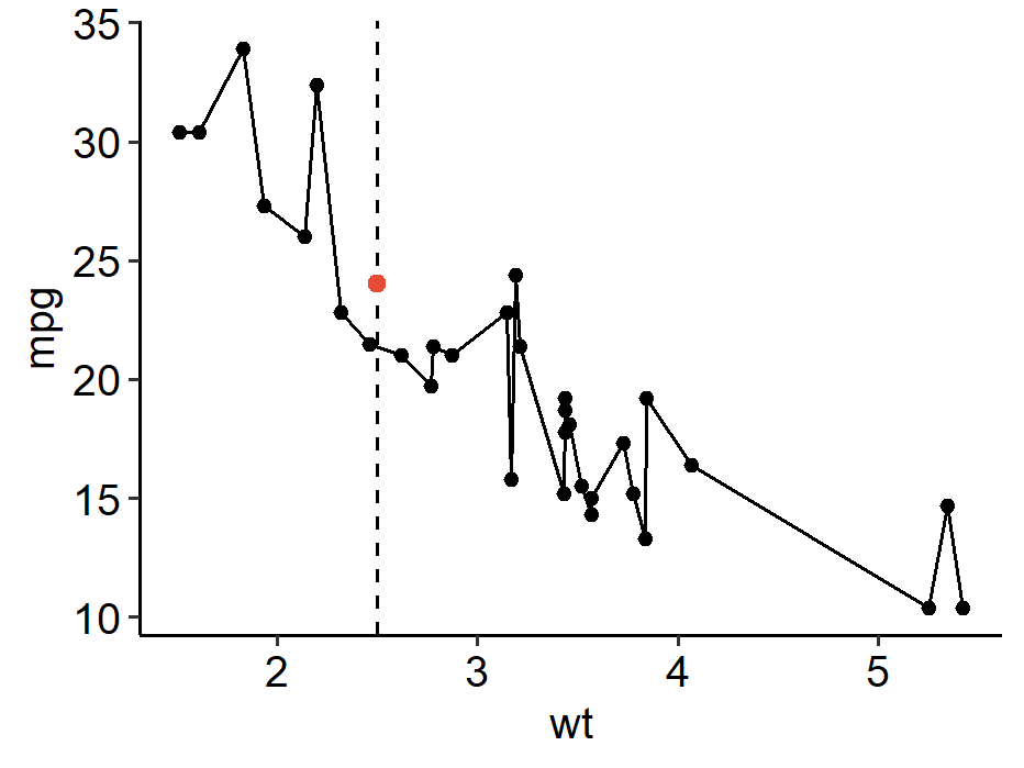
Suppose we collect data points $(x_i, y_i) \in \mathbb{R}^2$, $i = 1, \cdots, n$, and suspects a straight line relation $y = \beta_0 + \beta_1 x$. However, due to randomness, we very rarely see the points fall on a line perfectly. We can replace the line by a complex curve, but this yields bad predictions for new data1.

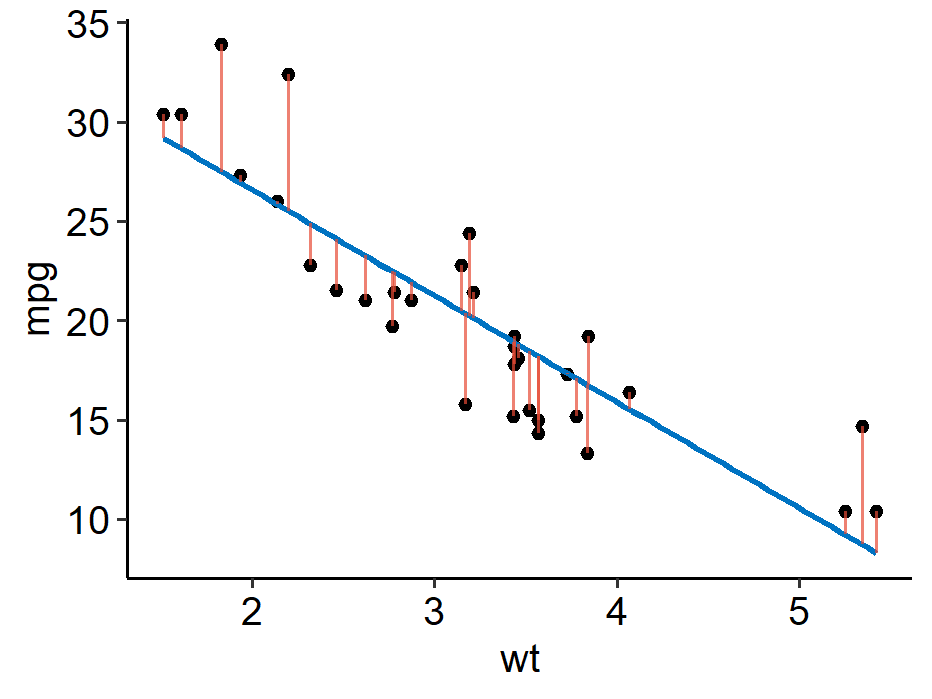
One often resorts to linear regression, whose geometric interpretation is to find a line that best fits the points according to certain criteria (e.g. least squares). The goal is to predict $y$ given a new $x$, or to understand how $x$ influences $y$. Clearly the $y_i$’s may not be identically distributed, and in fact we think they might depend on $x$2.

From a statistical modeling perspective, we assume a model
$$ \begin{equation}\label{eq:slr} Y_i = \beta_0 + \beta_1 x_i + \epsilon_i, \quad i = 1, \cdots, n \end{equation} $$
where $\epsilon_i$ is the random error term with mean $0$, and the intercept $\beta_0$ and slope $\beta_1$ are unknown parameters. Now fitting a line is equivalent to estimating $(\beta_0, \beta_1)$. We can also consider confidence intervals and hypothesis tests for them.
In statistical modeling, whenever the data is messy and don’t follow some deterministic relation, we often add in some random perturbation to relax our assumption.
Remark: We shall mostly treat $x_i$ as deterministic in this course. Depending on the context, one may also treat $x_i = X_i$ as random variables, typically independent of $\epsilon_i$.
Linear models
First we need to introduce some terminology and definitions.
Definitions
The $Y$ in Equation $\eqref{eq:slr}$ is called the response variable or dependent variable, and $x_1, \cdots, x_k$ are called independent variables or explanatory variables.
A linear model is given by
$$ \begin{equation}\label{eq:linear-model} E[Y] = \beta_0 + \beta_1 x_1 + \cdots + \beta_k x_k \Leftrightarrow Y = \beta_0 + \beta_1 x_1 + \cdots + \beta_k x_k + \epsilon \end{equation} $$
where $\epsilon$ is a random variable with $E[\epsilon] = 0$. When $k=1$, we have a simple linear regression (SLR) model.
If samples are indexed by $i = 1, \cdots, n$, the relation for the $i^{th}$ sample is written as
$$ Y_i = \beta_0 + \beta_1 x_{i1} + \cdots + \beta_k x_{ik} + \epsilon_i $$
Often we assume $\epsilon_i$ are i.i.d. with mean $0$ and variance $\sigma^2$ (typically unknown), or in addition $\epsilon_i \sim N(0, \sigma^2)$.
An observation is if the $x_i$’s are fixed, then $E[Y]$ is a linear function3 of $(\beta_0, \cdots, \beta_k)$. Here the “linear” is in terms of the coefficients $(\beta_0, \cdots, \beta_k)$, not the independent variables $(x_1, \cdots, x_k)$.
For example, all following models are linear models:
$$ \begin{gather*} Y = \beta_0 + \beta_1 x_1^2 + \beta_2 e^{x_2} + \epsilon \\ Y = \beta_1 x_1 + \beta_2 x_1^2 + \epsilon \\ Y = \beta_1 x_1 + \beta_1 x_1 x_2 + \epsilon \\ Y = (\beta_1 + \beta_2) \ln(x_1) + (\beta_1 - \beta_2)|x_2| \end{gather*} $$
because we can simply introduce new independent variables to get the model in the form of Equation $\eqref{eq:linear-model}$. For the first model we may take $x_1’ = x_1^2$ and $x_2’ = e^{x_2}$, then $Y = \beta_0 + \beta_1 x_1’ + \beta_2 x_2’ + \epsilon$.
The model
$$ Y = \beta_1 \beta_2 x_1 + (\beta_1 + \beta_2)x_2 + \epsilon $$
is nonlinear. In the remaining sections, we mainly focus on the simple linear regression case.
Least squares estimator
Given sample $(x_i, y_i)$, $i = 1, \cdots, n$, from the simple linear model $\eqref{eq:slr}$ the least squares estimator of $(\beta_0, \beta_1)$ is given by
$$ (\hat\beta_0, \hat\beta_1) = \underset{\beta_0, \beta_1}{\arg\min}\sum_{i=1}^n \left[y_i - (\beta_0 + \beta_1 x_i)\right]^2 $$
namely we want to find $(\beta_0, \beta_1)$ which minimizes the sum of squared errors (SSE) between the observation $y_i$ and the fitted value $\beta_0 + \beta_1 x_i$.
Proposition: The least squares solution is given by
$$ \begin{gather*} \hat\beta_1 = \frac{S_{xy}}{S_{xx}} = \frac{\sum_{i=1}^n (x_i - \bar{x})(y_i - \bar{y})}{\sum_{i=1}^n (x_i - \bar{x})^2} = \frac{\sum_{i=1}^n (x_i - \bar{x})y_i}{S_{xx}} \\ \hat\beta_0 = \bar{y} - \hat\beta_1 \bar{x} \end{gather*} $$
This can be found by partial derivations. If we denote the fitted value of the response at $x_i$ as
$$ \hat{y}_i = \hat\beta_0 + \hat\beta_1 x_i $$
and denote the residual $\hat\epsilon_i = y_i - \hat{y}_i$, which can be positive or negative. The expression for the SSE is
$$ SSE = \sum_{i=1}^n \hat\epsilon_i^2 = S_{yy} - \hat\beta_1S_{xy} $$
If one of the $\beta_i$’s is known, we can derive that
- When $\beta_1$ is known, $\hat\beta_0 = \bar{y} - \beta_1 \bar{x}$.
- When $\beta_0$ is known, $\hat\beta_1 = \frac{\sum_i x_i(y_i - \beta_0)}{\sum_i x_i^2}$.
Properties of the LSE
We now discuss the properties of the least squares estimator in a simple linear regression setting. Throughout the section, we assume the random errors $\epsilon_i$’s are i.i.d. with mean $0$ and variance $\sigma^2$. The lease squares estimator not only has nice geometric intuitions, but also some statistical properties.
Theorem: The least squares estimator $(\hat\beta_0, \hat\beta_1)$ in a simple linear regression satisfies the following:
$$ \begin{gather*} \text{Unbiasedness:} \quad E[\hat\beta_i] = \beta_i, \quad i = 1, 2 \\ Var(\hat\beta_1) = \frac{\sigma^2}{S_{xx}}, \quad Var(\hat\beta_0) = \frac{\sigma^2}{S_{xx}} \frac{\sum_{i=1}^n x_i^2}{n} \\ Cov(\hat\beta_0, \hat\beta_1) = -\frac{\sigma^2}{S_{xx}}\bar{x} \Rightarrow Cor(\hat\beta_0, \hat\beta_1) = \frac{Cov(\hat\beta_0, \hat\beta_1)}{\sqrt{Var(\hat\beta_0) Var(\hat\beta_1)}} = -\frac{\bar{x}}{\sqrt{\sum_{i=1}^n x_i^2/n}} \end{gather*} $$
The $S_{xx}$ quantity, known as the
leverage, measures how spread out the $x$ variable is.
The variances (MSEs) of the estimators are proportional to $\sigma^2$. Typically as we collect more data, $S_{xx} \rightarrow \infty$ and $\frac{\sum_{i=1}^n x_i^2}{n}$ stabilizes by the LLN, so we get consistency. We can also see the $\hat\beta_0$ and $\hat\beta_1$ are generally correlated unless $\bar{x} = 0$.
Proof for unbiasedness
First note that
$$ E[y_i] = E[\beta_0 + \beta_1 x_i + \epsilon_i] = \beta_0 + \beta_1 x_i + 0 $$
and
$$ \sum_{i=1}^n (x_i - \bar{x}) = 0, \quad S_{xx} = \sum_{i=1}^n (x_i - \bar{x})x_i, \quad S_{xy} = \sum_{i=1}^n (x_i - \bar{x})y_i $$
So by linearity of the expectations, we can expand these equations and get
$$ \begin{aligned} E[\hat\beta_1] &= E\left[\frac{\sum_{i=1}^n (x_i - \bar{x})y_i}{S_{xx}}\right] = \frac{\sum_{i=1}^n (x_i - \bar{x}) E[y_i]}{S_{xx}} \\ &= \frac{\sum_{i=1}^n (x_i - \bar{x})(\beta_0 + \beta_1 x_i)}{S_{xx}} = \frac{0 + \beta_1 S_{xx}}{S_{xx}} = \beta_1 \end{aligned} $$
The other part is much simpler:
$$ E[\hat\beta_0] = E[\bar{y}] - E[\hat\beta_1]\bar{x} = \beta_0 + \beta_1 \bar{x} - \beta_1 \bar{x} = \beta_0 $$
Estimator of the variance
An unbiased estimator of $\sigma^2$, the variance of the error term $\epsilon$, is given by
$$ \hat\sigma^2 = \frac{SSE}{n-2} = \frac{\sum_{i=1}^n (Y_i - \hat{Y}_i)^2}{n-2} $$
where the $n-2$ in the denominator is often interpreted as losing 2 degrees of freedom when estimating $\beta_0$ and $\beta_1$. Since we’re using $\hat{Y}_i$ to estimate $E[Y_i]$, it’s natural to estimate $\sigma^2$ based on the SSE.
$$ \begin{aligned} E[SSE] &= E\left[ \sum_{i=1}^n (Y_i - \hat{Y}i)^2 \right] = E\left[ \sum{i=1}^n(Y_i - \hat\beta_0 - \hat\beta_1 x_i)^2 \right] \\ &= E\left[ \sum_{i=1}^n (Y_i - \bar{Y} + \hat\beta_1 \bar{x} - \hat\beta_1 x_i)^2 \right] \\ &= E\left[ \sum_{i=1}^n [(Y_i - \bar{Y}) - \hat\beta_1 (x_i - \bar{x})]^2 \right] \\ &= E\left[ \sum_{i=1}^n (Y_i - \bar{Y})^2 + \hat\beta_1^2 \sum_{i=1}^n (x_i - \bar{x})^2 - 2\hat\beta_1 \sum_{i=1}^n (x_i - \bar{x})(Y_i - \bar{Y}) \right] \\ \end{aligned} $$
Note that
$$ \sum_{i=1}^n (x_i - \bar{x})(Y_i - \bar{Y}) = S_{xy} = S_{xx} \hat\beta_1 = \hat\beta_1 \sum_{i=1}^n (x_i - \bar{x})^2 $$
so the last two terms can be combined.
$$ \begin{aligned} E[SSE] &= E\left[ \sum_{i=1}^n (Y_i - \bar{Y})^2 - \hat\beta_1^2 \sum_{i=1}^n (x_i - \bar{x})^2 \right] \\ &= E\left[ \sum_{i=1}^n Y_i^2 - n\bar{Y}^2 - \hat\beta_1^2 \sum_{i=1}^n (x_i - \bar{x})^2 \right] \\ &= \sum_{i=1}^n E[Y_i^2] - nE[\bar{Y}^2] - S_{xx}E[\hat\beta_1^2] \\ &= \sum_{i=1}^n \left(Var(Y_i) + E[Y_i]^2 \right) - n\left(Var(\bar{Y}) + E[\bar{Y}]^2 \right) \\ &\qquad - S_{xx}\left(Var(\hat\beta_1) + E[\hat\beta_1]^2\right) \\ &= n\sigma^2 + \sum_{i=1}^n(\beta_0 + \beta_1 x_i)^2 - n\left(\frac{\sigma^2}{n} + (\beta_0 + \beta_1 \bar{x})^2\right) \\ &\qquad - S_{xx}\left(\frac{\sigma^2}{S_{xx}} + \beta_1^2\right) \\ &= (n-2)\sigma^2 \end{aligned} $$
Further assumptions
Theorem: If we assume in addition that the $\epsilon_i$’s are i.i.d. $N(0, \sigma^2)$, then
- $\hat\beta_0$ and $\hat\beta_1$ are normally distributed.
- $\frac{SSE}{\sigma^2} \sim \chi^2(n-2)$.
- SSE (hence $\hat\sigma^2$) is independent of $(\hat\beta_0, \hat\beta_1)$.
- In the MLE $(\hat\beta_0, \hat\beta_1, \hat\sigma^2)$, the former two coincides with the least squares estimate. Hint: $Y_i$’s are normally distributed and are independent of each other (not identically distributed because they depend on the $x_i$’s).
Inference of $\beta_0$ and $\beta_1$
So how can we directly make use of these properties to guide us make inference about $\beta_0$ and $\beta_1$? Specifically, we want to perform hypothesis testing or construct confidence intervals on $\beta_0$ and $\beta_1$.
An idea is that we know the formula for the variances of the estimators:
$$ Var(\hat\beta_1) = \frac{\sigma^2}{S_{xx}}, \quad Var(\hat\beta_0) = \frac{\sigma^2}{S_{xx}} \frac{\sum_{i=1}^n x_i^2}{n} $$
We may estimate $\hat\sigma$ using a Z-type test statistic. Take the following two-sided test for one of the parameters as an example. Our hypotheses are
$$ H_0: \beta_i = \beta_{i0} \quad vs. \quad H_a: \beta_i \neq \beta_{i0} $$
The test statistic is
$$ T = \frac{\hat\beta_i - \beta_{i0}}{S.E.} = \frac{\hat\beta_i - \beta_{i0}}{\hat\sigma \sqrt{c_i}} $$
where
$$ \hat\sigma = \frac{SSE}{n-2}, \quad c_0 = \frac{\sum_{i=1]^n x_i^2}}{nS_{xx}}, \quad c_1 = \frac{1}{S_{xx}} $$
Under $H_0$, assuming $\epsilon_i \overset{i.i.d.}{\sim} N(0, \sigma^2)$, we have $T \sim t(n-2)$.
When we have a small sample, the rejection rule is
$$ |T| > t_\frac{\alpha}{2}(n-2) $$
When $n$ is large, even without the normal assumption on $\epsilon_i$, typically $T \overset{\cdot}{\sim}N(0, 1)$, so we have the rejection rule as $|T| > z_\frac{\alpha}{2}$. Note that $t(\nu) \approx N(0, 1)$ when $\nu$ is large, so the two situations reconcile.
We can then invert the hypothesis test above to get a two-sided CI:
$$ \hat\beta_i \pm t_\frac{\alpha}{2}(n-2)\hat\sigma \sqrt{c_i} $$
- ↩︎
1 2 3 4 5 6 7 8library(tidyverse) data(mtcars) ggplot(mtcars, aes(x = wt, y = mpg)) + geom_point() + geom_line() + geom_point(aes(x = 2.5, y = 24), color = "#E64B35", size = 2) + ggpubr::theme_pubr() - ↩︎
1
2
3
4
5
6
7
8
9
m <- lm(mpg ~ wt, data = mtcars) mtcars %>% mutate(Fitted = fitted(m)) %>% ggplot(aes(x = wt, y = mpg)) + geom_point() + geom_smooth(method = "lm", formula = y ~ x, se = F, color = "#0073C2") + geom_segment(aes(x = wt, y = mpg, xend = wt, yend = Fitted), color = "#E64B35", alpha = 0.7) + ggpubr::theme_pubr() A function $f$ is said to be linear if it satisfies $$ f(a_1v_1 + a_2v_2) = a_1 f(v_1) + a_2 f(v_2) $$ for scalars $a_1$, $a_2$ and vectors $v_1$, $v_2$. ↩︎
| Apr 18 | Likelihood Ratio Test | 7 min read |
| Apr 14 | Optimal Tests | 7 min read |
| Apr 09 | p-values | 6 min read |
| Apr 01 | Statistical Test | 13 min read |
| Apr 01 | Statistical Decision | 4 min read |
 Yi's Knowledge Base