Functions of Random Variables
Suppose we have random variables $X_1, \cdots, X_n$, and a real-valued function $U(X_1, \cdots, X_n)$. In this chapter, we’re only going to do one thing: introduce multiple methods to find the probability distribution of $U$. Any one of these methods can be employed to find the distribution , but usually one of the methods leads to a simpler derivation than the others. The “best” method varies from one application to another.
The method of distribution functions
The first way of finding the distribution of $U$ is using the definition directly.
$$ F_U(a) = P\{U \leq a\} = P\{ U(X_1, \cdots, X_n) \leq a \} $$ We can work this out in the following steps:
- Write out the distribution function of $U$:
$$ F_U(a) = P\{ U(X_1, \cdots, X_n) \leq a \} $$
Find the region of $X_1, \cdots, X_n$ such that $U(X_1, \cdots, X_n) \leq a$ and denote the region as $D$.
Integrate $f(X_1, \cdots, X_n)$ over $D$.
$$ F_U(a) = \int\int\limits_D \cdots \int f(x_1, \cdots, x_n)dx_1 \cdots dx_n $$
The hardest part of this method is finding the set $D$. We’ll gain some insight with some examples.
Sugar example
A company is selling sugar online. Suppose the amount of sugar it can sell per day is $Y$ tons, which is a continuous random variable with density function defined as
$$ f_Y(y) = \begin{cases} 2y, & 0 \leq y \leq 1 \\ 0, & \text{otherwise} \end{cases} $$
For each ton of sugar sold, the company can earn $\$300$. The daily operation cost is $\$100$. Find the probability distribution of the daily income of this company.
Solution: Let the random variable $X$ denote the daily profit in hundred dollars. We want to write $X$ as $g(Y)$ and find $F_X(a)$.
$$ \begin{aligned} X &= 3Y - 1 \\ F_X(a) &= P\{X \leq a\} \\ &= P\{ 3Y - 1 \leq a \} \\ D &= \{Y: 3Y - 1 \leq a\} \\ &= \left\{Y \leq \frac{a+1}{3}\right\} \\ F_X(a) &= \int\limits_{Y \leq \frac{a+1}{3}}f_Y(y)dy \\ &= \int_{-\infty}^\frac{a+1}{3} f_Y(y)dy \end{aligned} $$
If $\frac{a+1}{3} < 0$, $f_Y(y) = 0$ $\Rightarrow$ $F_X(a) = 0$. If $\frac{a+1}{3} > 1$, $f_Y(y) = 1$ $\Rightarrow$ $F_X(a) = 1$. When $0 \leq \frac{a+1}{3} \leq 1$,
$$ \begin{aligned} F_X(a) &= \int_0^\frac{a+1}{3} f_Y(y)dy \\ &= \int_0^\frac{a+1}{3} 2ydy \\ &= y^2 \bigg|_0^\frac{a+1}{3} \\ &= \frac{(a+1)^2}{9} \end{aligned} $$
Note that as $y$ ranges from $0$ to $1$, $u$ ranges from $-1$ to $2$, so the distribution function of $X$ is
$$ F_X(a) = \begin{cases} 0, & a < -1 \\ \frac{(a+1)^2}{9}, & -1 \leq a \leq 2 \\ 1, & a > 2 \end{cases} $$ The density function can also be calculated:
$$ f_X(x) = \frac{dF_X(a)}{da} = \begin{cases} 0, & a < -1 \text{ or } a > 2 \\ \frac{2}{9}(a+1), & -1 \leq a \leq 2 \end{cases} $$
Example of two variables
Suppose $Y_1$ and $Y_2$ are two continuous random variables with joint density function
$$ f(y_1, y_2) = \begin{cases} 3y_1, & 0 \leq y_2 \leq y_1 \leq 1 \\ 0, & \text{otherwise} \end{cases} $$ Find the density function of $U = Y_1 - Y_2$. Also use the density function of $U$ to find $E[U]$.
We first need to find $F_U(a)$ and use it to obtain the density function $f_U(u)$.
$$ F_U(a) = P\{U \leq a\} = P\{Y_1 - Y_2 \leq a\} $$
Now we need to find the region of $y_1$ and $y_2$. We know that $y_1 - y_2 \leq a$ and $0 \leq y_2 \leq y_1 \leq 1$, and $a$ is bounded between $0$ and $1$ due to the latter condition.
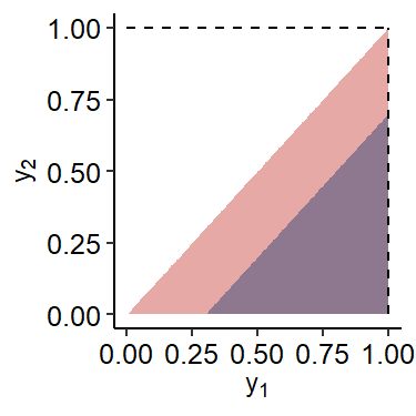
We can find the integral by subtracting the lower-right blue triangle region ($P\{U \geq a\}$) from the entire red triangle1.
$$ \begin{gather*} D = \{y_1, y_2: 0 \leq y_1 \leq 1, 0 \leq y_2 \leq y_1\} \\ F = \{y_1, y_2: a \leq y_1 \leq 1, 0 \leq y_2 \leq y_1 - a \} \end{gather*} $$
$$ \begin{aligned} F_U(a) &= \iint_D f(y_1, y_2)dy_1dy_2 - \iint_F f(y_1, y_2)dy_1dy_2 \\ &= 1 - \int_a^1 \int_0^{y_1 - a} f(y_1, y_2)dy_2 dy_1 \\ &= 1 - \int_a^1 dy_1 \int_0^{y_1 - a}3y_1 dy_2 \\ &= 1- \int_a^1 3y_1(y_1 - a) dy_1 \\ &= 1 - \left( y_1^3 - \frac{3}{2}ay_1^2 \right)\bigg|_a^1 \\ &= 1 - \left( 1 - \frac{3}{2}a - a^3 + \frac{3}{2}a^3 \right) \\ &= \frac{a}{2}\left(3-a^2\right),\quad 0 \leq a \leq 1 \end{aligned} $$
So the distribution function of $U$ is
$$ F_U(a) = \begin{cases} 0, & a < 0 \\ \frac{a}{2}\left(3-a^2\right), & 0 \leq a \leq 1 \\ 1, & a > 1 \end{cases} $$
Calculating the density function of $U$ is now straightforward:
$$ \begin{aligned} f_U(a) &= \frac{dF_U(a)}{da} = \frac{d\left[ \frac{3}{2}a - \frac{1}{2}a^3 \right]}{da} \\ &= \frac{3}{2} - \frac{3}{2}a^2 \\ &= \frac{3}{2}(1-a^2), \quad 0 \leq a \leq 1 \end{aligned} $$
which gives us
$$ f_U(u) = \begin{cases} \frac{3}{2}\left(1-u^2\right), & 0 \leq u \leq 1 \\ 0, & \text{otherwise} \end{cases} $$
The expectation of $U$ can be calculated as
$$ \begin{aligned} E[U] &= \int_0^1 u \cdot \frac{3}{2}(1-u^2)du \\ &= \int_0^1 \frac{3}{2}(u - u^3)du \\ &= \frac{3}{2}\left[ \frac{u^2}{2} - \frac{u^4}{4} \right] \bigg|_0^1 \\ &= \frac{3}{2} \cdot \frac{1}{4} = \frac{3}{8} \end{aligned} $$
Sum of independent random variables
An important application of the method of distribution functions is to calculate the distribution of $Z = X + Y$ from the distributions of $X$ and $Y$ when they are independent, continuous random variables.
The first few steps are the same as what’s described above:
$$ F_{X+Y}(a) = P\{X+Y \leq a\} = \iint\limits_{X+Y \leq a} f_{X,Y}(x, y)dxdy $$
Define the region $D$ such that
$$ D = \{x, y: -\infty < y < \infty, -\infty < x < a-y \} $$
We have
$$ \begin{aligned} F_{X+Y}(a) &= \iint\limits_D f_{X, Y}(x, y)dxdy \\ &= \int_{-\infty}^\infty \int_{-\infty}^{a-y}f(x, y)dxdy \end{aligned} $$
Now the independence comes into place:
$$ \begin{aligned} F_{X+Y}(a) &= \int_{-\infty}^\infty f_Y(y)dy \underbrace{\int_{-\infty}^{a-y}f_X(x)dx}{P\{X \leq a-Y\}} \\ &= \int{-\infty}^\infty F_X(a-y)f_Y(y)dy \end{aligned} $$
The distribution function of $F_{X+Y}(a)$ is called the convolution of $F_X(a)$ and $F_Y(a)$. By differentiating the above distribution function, we can find the density function of $X+Y$.
$$ \begin{aligned} f_{X+Y}(a) &= \frac{d}{da}\left\{ \int_{-\infty}^\infty F_X(a-y)f_Y(y)dy \right\} \\ &= \int_{-\infty}^\infty \frac{d}{da}F_X(a-y)f_Y(y)dy \\ &= \int_{-\infty}^\infty f_Y(y)dy \left[ \frac{d}{da}F_X(a-y) \right] \\ &= \int_{-\infty}^\infty f_Y(y)dy \left[ \frac{dF_X(a-y)}{d(a-y)}\frac{d(a-y)}{da} \right] \\ &= \int_{-\infty}^\infty f_Y(y) f_X(a-y)dy \end{aligned} $$
Uniform distribution example
If $X$ and $Y$ are two independent random variables both uniformly distributed on $(0, 1)$, calculate the probability density of $X+Y$. We can directly apply the equation above:
$$ \begin{gather*} f_{X+Y}(a) = \int_{-\infty}^\infty f_Y(y)f_X(a-y)dy \\ f_Y(y) = f_X(x) = \begin{cases} 1, & 0 \leq x \leq 1 \text{ or } 0 \leq y \leq 1 \\ 0, & \text{otherwise} \end{cases} \\ f_{X+Y}(a) = \int_0^1 1 \cdot f_X(a-y)dy \end{gather*} $$
We know that $0 \leq y \leq 1$ and $0 \leq a-y \leq 1$. There are several cases here:
- If $a \leq 0$, $a-y \leq 0$, then $f_X(a-y) = 0$.
- If $0 < a \leq 1$, we also need $a-y \geq 0$, or $0 \leq y \leq a$.
- If $1 < a \leq 2$, we also need $a-y \leq 1$, or $y \geq a-1$.
- If $a > 2$, $f_X(a-y) = 0$.
When $0 \leq a \leq 1$,
$$ f_{X+Y}(a) = \int_0^a f_X(a-y)dy = \int_0^ady = a $$
When $1 \leq a \leq 2$,
$$ f_{X+Y}(a) = \int_{a-1}^1 f_X(a-y)dy = 2-a $$
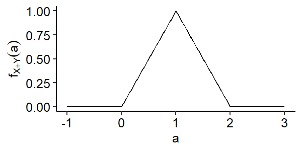
In summary,
$$ f_{X+Y}(a) = \begin{cases} a, & 0 < a \leq 1 \\ 2-a, & 1 < a \leq 2 \\ 0, & \text{otherwise} \end{cases} $$
The sum of two uniform random variables is called a triangular random variable because of the shape of the density function above2.
Normal distribution example
Suppose $X$ and $Y$ are two independent standard normal random variables. Find the density of $Z = X + Y$. Recall that
$$ f_X(x) = \frac{1}{\sqrt{2\pi}} e^{-\frac{x^2}{2}}, f_Y(y) = \frac{1}{\sqrt{2\pi}} e^{-\frac{y^2}{2}} $$
$$ \begin{aligned} f_{X+Y}(a) &= \int_{-\infty}^\infty f_X(a-y)f_Y(y)dy \\ f_X(a-y)f_Y(y) &= \frac{1}{2\pi}e^{-\frac{(a-y)^2}{2} - \frac{y^2}{2}} \\ &= \frac{1}{2\pi} \exp\left\{ -\frac{a^2 - 2ay + 2y^2}{2} \right\} \\ &= \frac{1}{2\pi} \exp\left\{ -\frac{4y^2 - 4ay + 2a^2}{4} \right\} \\ &= \frac{1}{2\pi} \exp\left\{ -\frac{(2y-a)^2 + a^2}{4} \right\} \\ &= \underbrace{\frac{1}{2\pi} \exp\left\{ -\frac{a^2}{4} \right\}}{\text{constant w.r.t. }y} \exp\left\{ -\frac{(2y-a)^2}{4} \right\} \\ f{X+Y}(a) &= \frac{1}{2\pi}\exp\left\{-\frac{a^2}{4}\right\} \int_{-\infty}^\infty \exp\left\{ -\frac{(2y-a)^2}{4} \right\}dy \\ &= C \cdot \exp\left\{-\frac{a^2}{4}\right\} \end{aligned} $$
Therefore $X+Y$ is a normal random variable with mean 0 and variance 2. Similar results of this example can be obtained for a more general case, which is a very important property of normal random variables.
Theorem
Let $X_i$, $i = 1, \cdots, n$ be a sequence of independent normal random variables with parameters $\mu_i$ and $\sigma_i^2$, then $\sum_{i=1}^n X_i$ is normally distributed with parameters $\sum_{i=1}^n \mu_i$ and $\sum_{i=1}^n \sigma_i^2$.
$$ \sum_{i=1}^n X_i \sim N\left( \sum_{i=1}^n \mu_i, \sum_{i=1}^n \sigma_i^2 \right) $$
The method of transformations
We first consider the univariate case. Suppose $X$ is a continuous random variable with density function $f_X(x)$. To find
$$ Y = g(X) \Rightarrow F_Y(a) $$
what we can do is to transform the condition back to a condition of $X$. We know that $g^{-1}(x)$ exists when the function $g(\cdot)$ is monotonic, i.e. $\forall x_1 \neq x_2$, $g(x_1) \neq g(x_2)$.
Given $g(x)$ is a monotonic function of $X$, $g(\cdot)$ maps every distinct value of $X$ to a distinct value of $y$.
If $g(\cdot)$ is a monotonically increasing function,
$$ \begin{gather*} F_Y(a) = P\{g(X) \leq a\} = P\left\{ X \leq g^{-1}(a) \right\} = F_X\left( g^{-1}(a) \right) \\ f_Y(a) = \frac{dF_Y(a)}{da} = \frac{dF_X(g^{-1}(a))}{dg^{-1}(a)} \cdot \frac{dg^{-1}(a)}{da} = f_X(g^{-1}(a))\frac{dg^{-1}(a)}{da} \end{gather*} $$
If $g(\cdot)$ is a monotonically decreasing function,
$$ \begin{gather*} F_Y(a) = P\{g(X) \leq a\} = P\left\{ X \geq g^{-1}(a) \right\} = 1- F_X\left( g^{-1}(a) \right) \\ f_Y(a) = \frac{d[1-F_X(g^{-1}(a))]}{da} -\frac{dF_Y(a)}{da} = f_X(g^{-1}(a))\left[-\frac{dg^{-1}(a)}{da}\right]\end{gather*} $$
These two cases can be unified as follows using the difference in the sign of $\frac{dg^{-1}(a)}{da}$. If $g(X)$ is a monotonic function for all $x$ such that $f_X(x) > 0$,
$$ f_Y(a) = f_X\left( g^{-1}(a) \right) \left| \frac{dg^{-1}(a)}{da} \right| $$
Sugar example revisited
In the sugar example, we defined the density function of $Y$ as
$$ f_Y(y) = \begin{cases} 2y, & 0 \leq y \leq 1 \\ 0, & \text{otherwise} \end{cases} $$
and $U = g(Y) = 3Y-1$. Find $f_U(u)$ with the method of transformations.
When $y_1 < y_2$,
$$ g(y_1) - g(y_2) = 3(y_1 - y_2) < 0 $$
so $g(\cdot)$ is a monotonically decreasing function. The inverse function is
$$ Y = g^{-1}(U) = \frac{U+1}{3} $$
and the first derivative is
$$ \frac{dg^{-1}(u)}{du} = \frac{d\frac{u+1}{3}}{du} = \frac{1}{3} $$
Now we can find the density function using the formula
$$ \begin{aligned} f_U(u) &= f_Y(g^{-1}(u)) \left| \frac{dg^{-1}(u)}{du} \right| \\ &= f_Y\left( \frac{u+1}{3} \right) \cdot \frac{1}{3} \\ &= 2\left(\frac{u+1}{3}\right) \cdot \frac{1}{3}, \quad 0 \leq \frac{u+1}{3} \leq 1 \end{aligned} $$
Clean this up a bit and we get
$$ f_U(u) = \begin{cases} \frac{2}{9}(u+1), & -1 \leq u \leq 2 \\ 0, & \text{otherwise} \end{cases} $$
Multivariate example
The transformation method can also be used in multivariate situations. Let random variables $Y_1$ and $Y_2$ have a joint density function
$$ f(y_1, y_2) = \begin{cases} e^{-(y_1 + y_2)}, & y_1 \geq 0, y_2 \geq 0 \\ 0, & \text{otherwise} \end{cases} $$
Find the density function for $U = Y_1 + Y_2$.
We can prove that $Y_1 \perp Y_2$ and use the method described earlier to find the distribution for the sum of two independent random variables. We can also apply the method of transformations here. If we fix $Y_1 = y_1$, we have
$$ U = g(Y_1, Y_2) = y_1 + Y_2 = h(Y_2) $$
From here we can consider this as a one-dimensional transformation problem.
$$ \begin{aligned} Y_2 &= U - y_1 = h^{-1}(u) \\ f_{Y_1, U}(y_1, u) &= f_{Y_1, Y_2}\left[y_1, h^{-1}(u) \right] \left| \frac{dg^{-1}(u)}{du} \right| \\ &= e^{-(y_1 + u - y_1)} \cdot 1 \\ &= e^{-u}, \quad y_1 \geq 0, \quad y_2 = u - y_1 \geq 0 \end{aligned} $$ Which is
$$ f_{U, Y_1}(u, y_1) = \begin{cases} e^{-u}, & 0 \leq y_1 \leq u \\ 0, & \text{otherwise} \end{cases} $$
Using the joint density function of $Y_1$ and $U$, we can obtain the marginal density function of $U$:
$$ \begin{aligned} f_U(u) &= \int_{-\infty}^\infty f_{U, Y_1}(u, y_1)dy_1 \\ &= \int_0^u e^{-u}dy_1 \\ &= ue^{-u}, \quad u \geq 0 \end{aligned} $$
So our final answer is
$$ f_U(u) = \begin{cases} ue^{-u}, & u \geq 0 \\ 0, & \text{otherwise} \end{cases} $$
Multivariate procedure
As shown in the example above, when our problem is $U = g(X_1, X_2)$ and we want to find $f_U(u)$, the procedure is
- Fix $X_1 = x_1$, and denote
$$ U|_{X_1 = x_1} = h(X_2) = g(X_1 = x_1, X_2) $$
- Calculate the joint density function of $X_1$ and $U$ using the formula
$$ f_{X_1, U}(x_1, u) = f_{X_1, X_2}\big(x_1, h^{-1}(u) \big)\left| \frac{dh^{-1}(u)}{du} \right| $$
- Find the marginal density of $U$ with
$$ f_U(u) = \int_{-\infty}^\infty f_{X_1, U}(x_1, u)dx_1 $$
Suppose random variables $Y_1$ and $Y_2$ have a joint density function
$$ f(y_1, y_2) = \begin{cases} 2(1-y_1), & 0 \leq y_1 \leq 1, 0 \leq y_2 \leq 1 \\ 0, & \text{otherwise} \end{cases} $$
Find the density function of $U = Y_1Y_2$.
Following the procedure, we first fix $Y_1 = y_1$ for some $0 \leq y_1 \leq 1$. Then we consider the univariate transformation $U = h(Y_2) = y_1Y_2$ and get the joint density function for $Y_1$ and $U$.
$$ \begin{aligned} U|{Y_1 = y_1} &= g(Y_1 = y_1, Y_2) = y_1Y_2 = h(Y_2) \\ Y_2 &= h^{-1}(U) = \frac{u}{y_1}, \frac{dh^{-1}(u)}{du} = \frac{1}{y_1} \\ f{Y_1, U}(y_1, u) &= f_{Y_1, Y_2}(y_1, h^{-1}(u))\left| \frac{dh^{-1}(u)}{du} \right| \\ &= 2(1-y_1) \cdot \frac{1}{y_1}, \quad 0 < y_1 \leq 1, \quad 0 \leq y_2 = \frac{u}{y_1} \leq 1 \end{aligned} $$
The joint density function of $Y_1$ and $U$ is
$$ f_{Y_1, U} = \begin{cases} \frac{2}{y_1}(1-y_1), & 0 < y_1 \leq 1, 0 \leq u \leq y_1 \\ 0, & \text{otherwise} \end{cases} $$
and now we can obtain the marginal density of $U$:
$$ \begin{aligned} f_U(u) &= \int_{-\infty}^\infty f_{Y_1, U}(y_1, u)dy_1 \\ &= \int_u^1 \frac{2}{y_1}(1-y_1) dy_1 \\ &= 2\int_u^1 \left( \frac{1}{y_1} - 1 \right)dy_1 \\ &= 2[\ln(y_1) - y_1]\bigg|_u^1 \\ &= 2[(0 - 1) - (\ln(u) - u)] \\ &= 2[u - \ln(u) - 1], \quad 0 \leq u \leq 1 \end{aligned} $$
The method of moment generating functions
We know that for a random variable $X$, its associated moment generating functions $M_X(t)$ is given by $E\left[e^{tX}\right]$. The $k^{th}$ moment can help us find $E[X^k] = M_X^{(k)}(0)$.
For random variables $X$ and $Y$, if both moment generating functions exist and $M_X(t) = M_Y(t)$, we have $F_X(a) = F_Y(a)$, i.e. $X$ and $Y$ have the same probability distribution.
Normal random variables
Let $Z \sim N(0, 1)$ and $X = \sigma Z + \mu$. Show that $X \sim N(\mu, \sigma^2)$ using the method of moment generating functions.
Define $Y \sim N(\mu, \sigma^2)$. If we can show that $M_X(t) = M_Y(t)$, then the distribution of $X$ is identical to the distribution of $Y$.
$$ \begin{aligned} M_Y(t) &= E\left[ e^{tY} \right] = \int_{-\infty}^\infty e^{ty}f_Y(y)dy \\ &= \exp\left\{ \frac{\sigma^2 t^2}{2} + \mu t \right\} \\ M_X(t) &= E\left[ e^{tX} \right] = E\left[ e^{t(\sigma Z + \mu)} \right] \\ &= E\left[ e^{t\mu}e^{(t\sigma)Z} \right] \\ &= e^{t\mu} E\left[ e^{(t\sigma)Z} \right] \\ &= e^{t\mu} M_Z(t\sigma) \end{aligned} $$
We know that $M_Z(t) = \exp\left\{ \frac{t^2}{2} \right\}$, so
$$ \begin{aligned} M_X(t) &= e^{t\mu} e^{\frac{\sigma^2t^2}{2}} \\ &= \exp\left\{ \frac{\sigma^2t^2}{2} + \mu t \right\} = M_Y(t) \end{aligned} $$
Use for sum of independent random variables
The method of moment generating functions is also very useful for calculating the probability distributions for the sum of independent random variables.
Suppose $X$ and $Y$ are independent with moment generating functions $M_X(t)$ and $M_Y(t)$. If $U = X + Y$, then
$$ \begin{aligned} M_U(t) &= E\left[e^{tU}\right] = E\left[e^{t(X+Y)}\right] \\ &= E\left[\underbrace{e^{tX}}_{g(X)} \cdot \underbrace{e^{tY}}_{h(Y)}\right] \\ &= E\left[e^{tX}\right]E\left[e^{tY}\right] = M_X(t) \cdot M_Y(t) \end{aligned} $$
In this special case,
$$ X \perp Y \Leftrightarrow M_{X+Y}(t) = M_X(t) M_Y(t) $$
Some more examples
Find the distribution of $X+Y$ if $X$ and $Y$ are
- independent binomial random variables with parameters $(n, p)$ and $(m, p)$, respectively.
- independent Poisson random variables with parameters $\lambda_1$ and $\lambda_2$, respectively.
In the first scenario we have $X \sim Bin(n, p)$ and $Y \sim Bin(m, p)$. $M_{X+Y}(t) = M_X(t)M_Y(t)$ since $X \perp Y$. Recall that
$$ M_X(t) = \left(pe^t + 1 - p \right)^n $$
so the MGF of $X+Y$ is
$$ M_{X+Y}(t) = \left(pe^t + 1 - p \right)^{m+n} $$
which tells us $X+Y \sim Bin(m+n, p)$.
In the second case, we have $X \sim Pois(\lambda_1)$ and $Y \sim Pois(\lambda_2)$. Since
$$ M_X(t) = \exp\left\{ \lambda(e^t - 1) \right\} $$
the MGF of $X+Y$ can be written as
$$ \begin{aligned} M_{X+Y}(t) &= \exp\{\lambda_1(e^t-1)\} \cdot \exp\{\lambda_2(e^t-1)\} \\ &= \exp\{(\lambda_1 + \lambda_2)(e^t-1)\} \end{aligned} $$ So $X+Y \sim Pois(\lambda_1 + \lambda_2)$.
- ↩︎
1 2 3 4 5 6 7 8 9 10 11 12 13library(ggplot2) ggplot(NULL, aes(x = c(0, 1))) + stat_function( fun = ~ .x - 0.3, geom = "area", xlim = c(0.3, 1), fill = "#0073C2", alpha = 0.7 ) + stat_function( fun = ~ .x, geom = "area", xlim = c(0, 1), fill = "#CD534C", alpha = 0.5 ) + geom_segment(aes(x = 1, y = 0, xend = 1, yend = 1), linetype = "dashed") + geom_segment(aes(x = 0, y = 1, xend = 1, yend = 1), linetype = "dashed") + labs(x = expression(y[1]), y = expression(y[2])) + ggpubr::theme_pubr() - ↩︎
1 2 3 4 5 6 7ggplot(NULL, aes(x = c(-1, 3))) + stat_function(fun = ~ 0, geom = "line", xlim = c(-1, 0)) + stat_function(fun = ~ .x, geom = "line", xlim = c(0, 1)) + stat_function(fun = ~ 2 - .x, geom = "line", xlim = c(1, 2)) + stat_function(fun = ~ 0, geom = "line", xlim = c(2, 3)) + labs(x = "a", y = expression(f[X+Y](a))) + ggpubr::theme_pubr()
| Dec 28 | Sampling Distribution and Limit Theorems | 6 min read |
| Nov 06 | Multivariate Probability Distributions | 23 min read |
| Nov 01 | Common Continuous Random Variables | 17 min read |
| Oct 06 | Common Discrete Random Variables | 14 min read |
| Oct 06 | Definitions for Discrete Random Variables | 7 min read |