Definitions for Discrete Random Variables
In this chapter, we restrict ourselves to study a special type of random variables - the discrete random variables.
When an experiment is performed, we are often interested in some functions of the outcomes, rather than the outcomes themselves. For example, when we toss two six-sided dice, we may care about the sum of the two dice. These real-valued functions defined on the sample space are known as random variables.
Probability mass function
A random variable is said to be discrete if it can take a finite or countable infinite number of distinct values. In practice, we usually use an uppercase letter to denote a random variable. For example,
$$
X: S \rightarrow \mathbb{R}
$$
and a lowercase letter, say $x$, to denote a possible value of this random variable. When we say $X = x$, we’re referring to the set of outcomes on the sample space such that $\{X = x\}$ holds. As an example,
$$
\begin{gather*}
X: \text{sum of two dice rolls} \\
\{X = 7\} = \{ (1, 6), (2, 5), \cdots, (6, 1) \}
\end{gather*}
$$
Then we can assign a probability to each of the events. The probability mass function (PMF) of a discrete random variable $X$ at a given value $x$ is denoted
$$
P\{X = x\} = p_X(x)
$$
The probability distribution of a discrete random variable $X$ is a collection of its probability mass functions over all its possible values. In other words, a collection of $p(x)$ for all $X$.
Coin flip example
Consider an experiment of tossing two fair coins. Denote $X$ as the number of heads. Find the probability distribution of $X$.
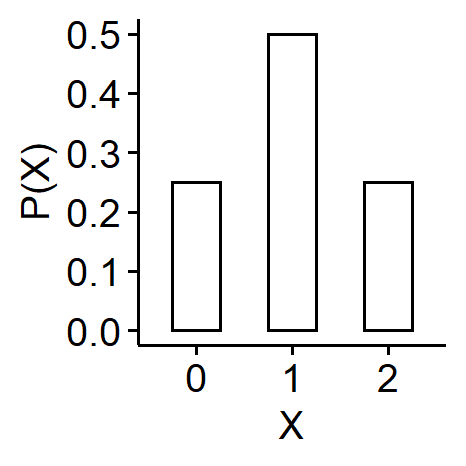
Our sample space is $$ S = \{ (H, H), (H, T), (T, H), (T, T) \} $$ For the random variable $X$: the number of heads, if we view $X$ as a function of $S$, $$ \begin{cases} X((H, H)) = 2 \\ X((H, T)) = 1 \\ X((T, H)) = 1 \\ X((T, T)) = 0 \end{cases} $$ $X$ can take three possible values: 0, 1 and 2. The probability mass functions are $$ \begin{aligned} p_X(0) &= P\{ X = 0 \} = P\{(T, T)\} = \frac{1}{4} \\ p_X(1) &= P\{ X = 1 \} = P\{(T, H), (H, T)\} = \frac{1}{2} \\ p_X(2) &= P\{ X = 2 \} = P\{(H, H)\} = \frac{1}{4} \end{aligned} $$ So the probability distribution of $X$ is given by $$ P(X) = \begin{cases} 0.25, & X = 0, 2 \\ 0.5, & X = 1 \end{cases} $$ Often a bar plot is used to show the probability distribution of $X$, with possible values of $X$ of the x-axis, and $P(X)$ on the y-axis.
| |
Properties
The PMF must satisfy certain properties. Suppose $X$ is a discrete random variable with possible values $X_1, X_2, \cdots$.
- $P(X_i) > 0$ $\forall X_i$ and $P(X) = 0$ $\forall$ other $X$, which is to say the probability must be greater than 0.
- $\sum_{i=1}^\infty P(X_i) = 1$.
- For all the possible outcomes of a random variable $X$ where $X_i \neq X_j$,
$$ \{X = X_i\} \cap \{ X = X_j\} = \emptyset $$
- For all the possible outcomes we also have
$$ \bigcup_{i=1}^n\{ X = X_i \} = S $$
For properties 3 and 4, we can think of each of $X_i$ as a simple event for the sample space $S$.
Cumulative distribution function
Besides the PMF which gives us the probability of one possible value of a random variable, we may want to calculate the probability for multiple values of a random variable. In the coin flip example,
$$
\begin{aligned}
P\{ X < 2 \} &= P\{ X = 1 \text{ or } 0 \} \\
&= P(\{X = 1\} \cup \{X = 0\}) \\
&= \sum_{i=0}^1P(i) = \frac{1}{4}+ \frac{1}{2} = \frac{3}{4}
\end{aligned}
$$
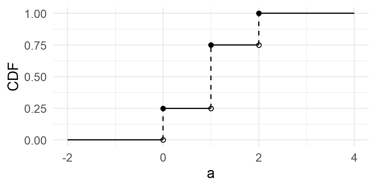
The cumulative distribution function (CDF) is defined as
$$
F(a) = P\{X \leq a\} = \sum_{x \leq a} p(x)
$$
under the discrete case. In the example above,
$$
P\{X < 2\} = P\{X \leq 1\} = F(1) = p(1) + p(0)
$$
In addition, we can write out the whole cumulative distribution function for all possible values of $a$
$$
F_X(a) = \begin{cases}
0, && a < 0 \\
\frac{1}{4}, && 0 \leq a < 1 \\
\frac{3}{4}, && 1 \leq a < 2 \\
1, && a \geq 2
\end{cases}
$$
The figure for the CDF of a discrete random variable is a non-decreasing step function of $a$. Given a data set in R, we can use the geom_step() function to visualize the CDF, or stat_ecdf() for the empirical distribution function (ECDF). Generating the following figure knowing the true CDF involves a bit more manual labor1.
Expected value
After we’ve learnt the PMF and the CDF, we can move one step further to probably one of the most important concepts in probability theory - the expectation of a random variable.
If $X$ is a discrete random variable with probability mass function $P(X)$, its expectation is
$$
E[X] = \sum_X{Xp(X)} = \sum_{X: p(X) > 0}{Xp(X)}
$$
Intuitively, it is the long-run average value of repetitions of the same experiment the random variable represents. In our case, the expected value of a discrete random variable is the probability-weighted average of all possible values.
Recall that random variables are some real-valued functions that map the outcomes in a sample space to some real numbers. So a real-valued function of a random variable is also a real-valued function on the same sample space, and hence is also a random variable.
Define $Y = g(X)$ with $g(\cdot)$ being a real-valued function. This means that everything we can perform on X can be done in a similar fashion on $Y$. For example, calculating the expected value of $Y$: $$ E[Y] = E[g(X)] = \sum_{g(X)}g(x)p(x) = \sum_{X:P(X) > 0}g(x)p(x) $$ The only difference between $E[X]$ and $E[Y]$ is we replace $X_i$ by $g(X_i)$ in the summation. Note how $p(x)$ wasn’t changed!
Since the expected value is a linear function, given $X$ is a random variable, $g(\cdot)$ and $h(\cdot)$ are two real-valued functions and $\alpha$ and $\beta$ are two constants, $$ E[\alpha g(X) + \beta h(X)] = \alpha E[g(X)] + \beta E[h(X)] $$
Variance
The variance of a random variable $X$ is often denoted $\sigma^2$, and can be written as the expectation of a function of $X$
$$
\begin{aligned}
Var(X) &= E\left[ (X - E[X] )^2 \right] \\
&= E\left[ X^2 - 2XE[X] + E[X]^2 \right] \\
&= E[X^2] - 2E[X]^2 + E[X]^2 \\
&= E[X^2] - (E[X])^2
\end{aligned}
$$
We’ll explain the two definitions through an example. Let $X$ be a discrete random variable with three possible values $-1, 0, 1$, and probability mass function
$$
P(-1) = 0.2, P(0) = 0.5, P(1) = 0.3
$$
Find $E(X)$ and $E(X^2)$. By definition, we have
$$
\begin{aligned}
E(X) &= \sum_X{XP(X)} \\
&= -1 \times P(-1) + 0 \times P(0) + 1 \times P(1) \\
&= -0.2 + 0.3 = 0.1
\end{aligned}
$$
Let $Y = g(X) = X^2$, we have
$$
\begin{aligned}
E(X^2) &= \sum_{X}X^2P(X) \\
&= (-1)^2P(-1) + 0^2P(0) + 1^2P(1) \\
&= 0.2 + 0.3 = 0.5
\end{aligned}
$$
- ↩︎
1 2 3 4 5 6 7 8 9 10 11 12 13 14 15 16 17 18 19 20 21library(ggplot2) library(dplyr) dat <- data.frame( a = rep(0:2, each = 2), CDF = c(0, 1/4, 1/4, 3/4, 3/4, 1), Group = rep(c("Empty", "CDF"), 3) ) ggplot(dat) + geom_point(aes(a, CDF, fill = Group), shape = 21) + scale_fill_manual(values = c("black", "white")) + geom_segment(aes( x = lag(a), y = lag(CDF), xend = a, yend = CDF, lty = Group )) + scale_linetype_manual(values = c("dashed", "solid")) + geom_segment(aes(x = -2, xend = 0, y = 0, yend = 0)) + geom_segment(aes(x = 2, xend = 4, y = 1, yend = 1)) + theme_minimal() + theme(legend.position = "none")
| Dec 28 | Sampling Distribution and Limit Theorems | 6 min read |
| Dec 08 | Functions of Random Variables | 14 min read |
| Nov 06 | Multivariate Probability Distributions | 23 min read |
| Nov 01 | Common Continuous Random Variables | 17 min read |
| Oct 06 | Common Discrete Random Variables | 14 min read |