Estimation

Introduction
We start by defining what a linear model is. Suppose we’re interested in the response $Y$ in terms of three predictors1, $X_1$, $X_2$ and $X_3$. One very general form for the model would be:
$$ Y = f(X_1, X_2, X_3) + \epsilon $$
where $f$ is some unknown function and $\epsilon$ is the error in this representation. Typically we don’t have enough data to estimate $f$ directly (even with just three predictors), so we usually have to assume that it has some more restricted form.
Linear model
One of the possibilities is perhaps a linear model:
$$ Y = \beta_0 + \beta_1 X_1 + \beta_2 X_2 + \beta_3 X_3 + \epsilon $$
where $\beta_i, i = 0, 1, 2, 3$ are unknown parameters, and $\beta_0$ is called the intercept term. The problem is thus reduced to the estimation of four parameters rather than the infinite dimensional $f$. In a linear model the parameters enter linearly, meaning that the predictors do not have to be linear.
In other words, linear models can be curved. For example, the following models are all linear models:
| Model type | Formula |
|---|---|
| Null model | $Y_i = \beta_0 + \epsilon_i$ |
| Simple linear model | $Y_i = \beta_0 + \beta_1 X_i + \epsilon_i$ |
| Quadratic model | $Y_i = \beta_0 + \beta_1 X_i + \beta_2 X_i^2 + \epsilon_i$ |
| Linear mixed model | $Y_i = \beta_0 + \beta_1 X_{i1} + \beta_2 X_{i2} + \epsilon_i$ |
| Mixed model w/ interaction | $Y_i = \beta_0 + \beta_1 X_{i1} + \beta_2 X_{i2} + \beta_3 X_{i1} X_{i2} + \epsilon$ |
| $Y_i = \beta_0 + \beta_1 X_{i1} + \beta_2 \log X_{i2} + \beta_3 X_{i1} X_{i2} + \epsilon$ |
However, this
$$ Y_i = \beta_0 + \beta_1 X_{i1}^{\beta_2} + \epsilon_i $$
is not a linear model. Some models can be transformed to linearity, for example
$$ Y_i = \beta_0 X_i^{\beta_1} \epsilon_i $$
can be linearized by taking logs.
Matrix representation
All of the models above can be expressed as a general linear model, provided that we can decide what the predictors and the parameters are. Suppose there’s $n$ observations in our data, we have:
$$ \begin{equation}\label{eq:linear-model-tabular} \begin{gathered} Y_1 = \beta_0 + \beta_1 X_{11} + \beta_2 X_{12} + \cdots + \beta_k X_{1k} + \epsilon_1 \\ Y_2 = \beta_0 + \beta_1 X_{21} + \beta_2 X_{22} + \cdots + \beta_k X_{2k} + \epsilon_2 \\ \vdots \\ Y_n = \beta_0 + \beta_1 X_{n1} + \beta_2 X_{22} + \cdots + \beta_k X_{nk} + \epsilon_n \end{gathered} \end{equation} $$
We want a general solution to estimating the parameters of a linear model. For some special cases (e.g. simple linear regression) a simple formulae can be found, but for a method that works in all cases we’ll need matrix algebra. The model in $\eqref{eq:linear-model-tabular}$ can be conveniently written in matrix notation as:
$$ \boldsymbol{y} = \boldsymbol{X\beta} + \boldsymbol{\epsilon} $$
where $\boldsymbol{y} = (y_1, \cdots, y_n)^\prime$, $\boldsymbol{\epsilon} = (\epsilon_1, \cdots, \epsilon_n)^\prime$, $\boldsymbol{\beta} = (\beta_0, \cdots, \beta_k)^\prime$ and
$$ \boldsymbol{X} = \begin{pmatrix} 1 & X_{11} & \cdots & X_{1k} \\ 1 & X_{21} & \cdots & X_{2k} \\ \vdots & \vdots & \ddots & \vdots \\ 1 & X_{n1} & \cdots & X_{nk} \end{pmatrix} $$
The column of ones incorporates the intercept term. In the null model where there’s no predictor, we simply have
$$ \begin{pmatrix} y_1 \\ \vdots \\ y_n \end{pmatrix} = \begin{pmatrix} 1 \\ 1 \\ 1 \end{pmatrix} \mu + \begin{pmatrix} \epsilon_1 \\ \vdots \\ \epsilon_n \end{pmatrix} $$
We can assume that $E[\boldsymbol{\epsilon}] = 0$ because otherwise we could just merge the non-zero expectation for the error term into the mean $\mu$.
Estimation
The unknown parameters in the model $\boldsymbol{y} = \boldsymbol{X\beta} + \boldsymbol{\epsilon}$ are the regression coefficient $\boldsymbol{\beta}$ and the error variance $\sigma^2$. The purpose of collecting the data is to estimate and make inferences about these parameters.
Estimating $\boldsymbol{\beta}$
The regression model partitions the response into a systematic component $X\beta$ and a random component $\epsilon$. We want to choose $\beta$ such that the systematic part explains as much of the response as possible, leaving just random variation in the residuals.
Geometrically speaking, the response $\boldsymbol{y}$ lies in an $n$-dimensional space ($\boldsymbol{y} \in \mathbb{R}^n$), while $\boldsymbol{\beta} \in \mathbb{R}^p$ where $n$ is the number of observations and $p$ is the number of parameters2.
To find $\boldsymbol{\beta}$ such that $\boldsymbol{X\beta}$ is as close to $Y$ as possible, we’d be looking for predicted/fitted values $\hat{Y}$ in $p$ dimensions that best represent the original $Y$, which is apparently found by projecting $Y$ orthogonally onto the model space spanned by $X$. The fitted values are found by
$$ \boldsymbol{\hat{Y}} = \boldsymbol{X\hat\beta} = \boldsymbol{HY} $$
where $H$ is an orthogonal projection matrix. $\hat\beta$, the regression coefficients, are the best estimates of $\beta$ within the model space. The difference between the actual response $Y$ and the predicted response $\hat{Y}$ is denoted by $\hat\epsilon$ and is called the residual.
Least squares estimation
The estimation of $\boldsymbol{\beta}$ can be considered from a nongeometric point of view. If we define the best estimate of $\boldsymbol{\beta}$ as the one which minimizes the sum of the squared errors:
$$ \sum\epsilon_i^2 = \boldsymbol{\epsilon^\prime\epsilon} = (\boldsymbol{ y - X\beta})^\prime(\boldsymbol{ y - X\beta}) $$
Expand this and we get
$$ \boldsymbol{y^\prime y} - 2\boldsymbol{\beta X^\prime y} + \boldsymbol{\beta^\prime X^\prime X \beta} $$
Differentiating with respect to $\boldsymbol{\beta}$ and setting to zero, we find that $\boldsymbol{\hat\beta}$ satisfies
$$ \boldsymbol{X^\prime X \hat\beta} = \boldsymbol{X^\prime y} $$
These are called the normal equations. Now if $\boldsymbol{X^\prime X}$ is invertible,
$$ \begin{aligned} \boldsymbol{\hat\beta} &= (\boldsymbol{X^\prime X})^{-1} \boldsymbol{X^\prime y} \\ \boldsymbol{X\hat\beta} &= \boldsymbol{X}(\boldsymbol{X^\prime X})^{-1} \boldsymbol{X^\prime y} \\ \boldsymbol{\hat{y}} &= \boldsymbol{Hy} \end{aligned} $$
where $\boldsymbol{H} = \boldsymbol{X}(\boldsymbol{X^\prime X})^{-1} \boldsymbol{X}^\prime$ is the $n \times n$ hat matrix and is the orthogonal projection of $\boldsymbol{y}$ onto the space spanned by $X$ mentioned above. The matrix is symmetric and idempotent. A few useful quantities can be represented using $H$:
- Predicted/fitted values: $\boldsymbol{\hat{y}} = \boldsymbol{Hy} = \boldsymbol{X\hat\beta}$
- Residuals: $\boldsymbol{\hat\epsilon} = \boldsymbol{y - X\hat\beta - y - \hat{y}} = (\boldsymbol{I-H})\boldsymbol{y}$
- Residual sum of squares (RSS): $\boldsymbol{\hat\epsilon^\prime\hat\epsilon} = \boldsymbol{y}^\prime(\boldsymbol{I-H})^\prime(\boldsymbol{I-H})\boldsymbol{y} = \boldsymbol{y}^\prime(\boldsymbol{I-H})\boldsymbol{y}$
Later we’ll show that the ordinary least squares (OLS) estimator is the best possible estimate of $\boldsymbol{\beta}$ when the errors are uncorrelated and have equal variance, i.e. $Var(\boldsymbol{\epsilon}) = \sigma^2\boldsymbol{I}$. $\boldsymbol{\hat\beta}$ is unbiased and has variance $(\boldsymbol{X^\prime X})^{-1} \sigma^2$.
$\boldsymbol{\hat\beta}$ is a good estimate from several aspects. First, it results from an orthogonal projection onto the model space, so it makes sense geometrically. Second, if the errors are independent and identically normally distributed, it’s the maximum likelihood estimator. Finally, the Gauss-Markov theorem states that it’s the best linear unbiased estimate (BLUE).
Estimation of $\sigma^2$
We found the RSS to be $\boldsymbol{\hat\epsilon^\prime\hat\epsilon} = \boldsymbol{y}^\prime(\boldsymbol{I-H})\boldsymbol{y}$. To find its expectation, we first rewrite the residual to be
$$ \boldsymbol{\hat\epsilon} = (\boldsymbol{I-H})\boldsymbol{y} = (\boldsymbol{I-H})\boldsymbol{X\beta} + (\boldsymbol{I-H})\boldsymbol{\epsilon} $$
The first part is zero because
$$ (\boldsymbol{I-H})\boldsymbol{X} = \boldsymbol{X} - \boldsymbol{X}(\boldsymbol{X^\prime X})^{-1} \boldsymbol{X}^\prime\boldsymbol{X} = \boldsymbol{X} - \boldsymbol{X} = 0 $$
Thus the RSS is
$$ \begin{aligned} RSS &= \boldsymbol{\epsilon}^\prime(\boldsymbol{I-H})^\prime(\boldsymbol{I-H})\boldsymbol{\epsilon} \\ &= \boldsymbol{\epsilon}^\prime(\boldsymbol{I-H})\boldsymbol{\epsilon} \\ &= \boldsymbol{\epsilon}^\prime\boldsymbol{\epsilon} - \boldsymbol{\epsilon}^\prime\boldsymbol{H\epsilon} \\ \end{aligned} $$
We know that the errors are i.i.d. with mean 0 and variance $\sigma^2$, so
$$ E[\epsilon_i \epsilon_j] = \begin{cases} 0, & i \neq j, \\ \sigma^2, & \text{otherwise} \end{cases} $$
So the expectation is
$$ \begin{aligned} E[RSS] &= E\left[ \boldsymbol{\epsilon}^\prime\boldsymbol{\epsilon} - \boldsymbol{\epsilon}^\prime\boldsymbol{H\epsilon} \right] \\ &= n\sigma^2 - E\left[ \boldsymbol{\epsilon}^\prime\boldsymbol{H\epsilon} \right] \\ &= n\sigma^2 - E\left[ Tr(\boldsymbol{\epsilon}^\prime\boldsymbol{H\epsilon}) \right] \\ &= n\sigma^2 - Tr(\boldsymbol{H})\sigma^2 \\ &= n\sigma^2 - Tr \left(\boldsymbol{X}(\boldsymbol{X}^\prime\boldsymbol{X})^{-1} \boldsymbol{X}^\prime \right) \sigma^2 \\ &= n\sigma^2 - Tr \left(\boldsymbol{X}(\boldsymbol{X}^\prime\boldsymbol{X}^\prime\boldsymbol{X})^{-1} \right) \sigma^2 \\ &= n\sigma^2 - Tr(\boldsymbol{I}_{p}) \sigma^2 \\ &= (n-p)\sigma^2 \end{aligned} $$
With this, we can easily see that
$$ \hat\sigma^2 = \frac{\boldsymbol{\hat\epsilon}^\prime \hat{\boldsymbol{\epsilon}}}{n-p} $$
is an unbiased estimator of $\sigma^2$. The $n-p$ here is reffered to as the degrees of freedom of the model.
Sometimes we need the standard error for a specific parameter, in this case we may look at the diagonal of the variance-covariance matrix:
$$ se(\hat\beta_{i-1}) = \sqrt{(\boldsymbol{X}^\prime \boldsymbol{X})_{ii}^{-1}} \hat\sigma $$
Gauss-Markov theorem
To understand the theorem, we first need the concept of an estimable function. A linear combination of the parameters $\Psi = c^\prime \beta$ is estimable if and only if there exists a linear combination of the observations $a^\prime y$ such that
$$ E\left[ a^\prime y \right] = c^\prime \beta \quad \forall \beta $$
If $X$ is of full rank, then all linear combinations are estimable3.
Suppose $E[\boldsymbol{\epsilon}] = 0$ and $Var(\boldsymbol{\epsilon} = \sigma^2\boldsymbol{I}$. Suppose also that the structural part of the model, $E[Y] = X\beta$, is correct. Let $\Psi = c^\prime \beta$ be an estimable function, then the Gauss-Markov theorem states that in the class of all unbiased linear estimates of $\Psi$, $\hat\Psi = c^\prime \hat\beta$ has the minimum variance and is unique.
Proof
Suppose $a^\prime y$ is some unbiased estimate of $c^\prime \beta$ such that
$$ \begin{gathered} E[a^\prime y] = c^\prime \beta \quad \forall \beta \\ a^\prime X\beta = c^\prime \beta \quad \forall \beta \end{gathered} $$
which means that $a^\prime X = c^\prime$. This implies $c$ must be in the column space of $X^\prime$, which in turn implies that $c$ is also in the column space of $X^\prime X$. This means there exists a $\lambda$ such that $c = X^\prime X \lambda$, so
$$ c^\prime \hat\beta = \lambda^\prime X^\prime X \hat\beta = \lambda^\prime X^\prime y $$
Now we can show that the LSE has the minimum variance. We may pick an arbitrary estimate $a^\prime y$ and compute its variance:
$$ \begin{aligned} Var(a^\prime y) &= Var \left( a^\prime y - c^\prime \hat\beta + c^\prime \hat\beta \right) \\ &= Var \left( a^\prime y - \lambda^\prime X^\prime y + c^\prime \hat\beta \right) \\ &= Var \left( a^\prime y - \lambda^\prime X^\prime y\right) + Var \left(c^\prime \hat\beta \right) + 2Cov \left( a^\prime y - \lambda^\prime X^\prime y, \lambda^\prime X^\prime y \right) \end{aligned} $$
If we focus on the covariance term:
$$ \begin{aligned} Cov \left( a^\prime y - \lambda^\prime X^\prime y, \lambda^\prime X^\prime y \right) &= Cov \left( (a^\prime - \lambda^\prime X^\prime)y, \lambda^\prime X^\prime y \right) \\ &= \left( a^\prime - \lambda^\prime X^\prime \right)X\lambda \sigma^2 \boldsymbol{I} \\ &= \left( a^\prime X - \lambda^\prime X^\prime X \right)\lambda \sigma^2 \boldsymbol{I} \\ &= \left( c^\prime - c^\prime \right)\lambda \sigma^2 \boldsymbol{I} \\ &= 0 \end{aligned} $$
So
$$ Var(a^\prime y) = Var \left( a^\prime y - \lambda^\prime X^\prime y\right) + Var \left(c^\prime \hat\beta \right) \geq Var \left(c^\prime \hat\beta \right) $$
In other words, $c^\prime \hat\beta$ has minimum variance. The equality holds only when $a^\prime - \lambda^\prime X^\prime = 0$, which means $a^\prime y = \lambda^\prime X^\prime y = c^\prime \hat\beta$, so the estimator is unique because it only occurs when $a^\prime y = c^\prime \hat\beta$.
Implications
The Gauss-Markov theorem shows that the LSE is a good choice, but it does require the errors to be uncorrelated and homoscedastic (have equal variance). Even if this is the case but the errors are non-normal, nonlinear or biased estimates may work better. The theorem doesn’t tell us to use the LSE all the time - it just strongly suggests it unless there’s some strong reason to do otherwise.
Situations where estimators other than ordinary least squares should be considered are:
- When the errors are correlated or have unequal variance, generalized least squares should be used.
- When the error distribution is long-tailed, robust estimates4 might be used.
- When the predictors are high correlated, biased estimates such as ridge regression might be preferable.
Goodness of fit
It’s useful to have some measure of how well the model fits the data. One common choice is $R^2$, the coefficient of determination or percentage of variance explained:
$$ R^2 = 1 - \frac{\sum(\hat{y}_i - y_i)^2}{\sum(y_i - \bar{y})^2} = 1 - \frac{RSS}{TSS} $$
where TSS stands for total sum of squares. $R^2$ ranges between 0 and 1, and values closer to 1 indicates better fits. An equivalent definition is
$$ R^2 = \frac{\sum(\hat{y}_i - \bar{y})^2}{\sum(y_i - \bar{y})^2} = \frac{\text{Regression SS}}{TSS} = corr^2(\hat{y}, y) $$
It should be noted that the first definition requires an intercept in the regression model. It has a null model with an intercept when the sum of squares is calculated.
So what is a good value of $R^2$? It really depends on the area of application. In biological and social sciences, variables tend to be much more weakly correlated with a lot of noise involved. an $R^2$ of 0.6 might be considered good. In physics and engineering where most data are gathered from closely controlled experiments, $R^2 = 0.6$ could be considered low.
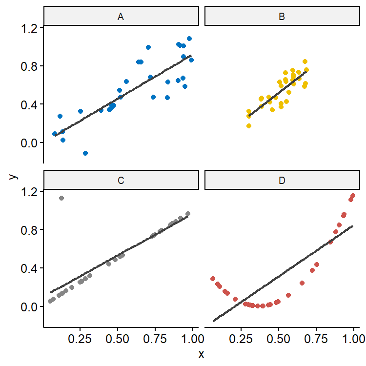
$R^2$ also shouldn’t be the sole measure of fit. As shown in Figure 15, although the $R^2$ is roughly 0.70 in all four simulated datasets, the underlying relationship could be very different. B has smaller variation in $x$ and also smaller residual variation compared with A, so predictions would also have less variation. C looks like a really good fit except for one outlier, demonstrating how sensitive $R^2$ is to extreme values. The true relationship in D seems to be quadratic, showing that $R^2$ doesn’t tell us much about whether we have the right model.
An alternative measure of fit is $\hat\sigma$. This quantity is directly related to the standard errors of estimates of $\beta$ and predictions. $\hat\sigma$ is measured in the unit of the response, so it can be directly interpreted given the context of the dataset, but it’s hard to say if a $\hat\sigma$ value is large or small as it depends on the scale of the data.
Simple linear regression
As we said earlier, in a few simple models it’s possible to derive explicit formulae for the parameter estimates. In the null model $y = \mu + \epsilon$, we have $\boldsymbol{X} = \boldsymbol{1}$ and $\beta = \mu$, hence
$$ \begin{gathered} \boldsymbol{X}^\prime \boldsymbol{X} = \boldsymbol{1}^\prime \boldsymbol{1} = n \\ \hat\beta = (\boldsymbol{X}^\prime \boldsymbol{X})^{-1} \boldsymbol{X}^\prime \boldsymbol{y} = \frac{1}{n}\boldsymbol{1}^\prime \boldsymbol{y} = \bar{y} \end{gathered} $$
In simple linear regression (SLR) where we have only one predictor, the model is
$$ \begin{equation} \label{eq:simple-linear-regression} y_i = \beta_0 + \beta_1 x_i + \epsilon_i \end{equation} $$
which in matrix notation is
$$ \begin{pmatrix} y_1 \\ \vdots \\ y_n \end{pmatrix} = \begin{pmatrix} 1 & x_1 \\ \vdots & \vdots \\ 1 & x_n \end{pmatrix} \begin{pmatrix} \beta_0 \\ \beta_1 \end{pmatrix} + \begin{pmatrix} \epsilon_1 \\ \vdots \\ \epsilon_n \end{pmatrix} $$
Here $x_i$ and $y_i$ are observed values, $\beta_0$ is the intercept, and $\beta_1$ is the slope. $\epsilon_i$ is the error for data pair $i$, and the $\epsilon$’s are assumed to be independent (frequently assumed normal) random variables with mean 0 and standard deviation $\sigma_\epsilon$.
Estimating parameters
We may apply the formula $\boldsymbol{\hat\beta} = (\boldsymbol{X^\prime X})^{-1} \boldsymbol{X^\prime y}$ directly, but a simpler approach is to rewrite $\eqref{eq:simple-linear-regression}$ as
$$ y_i = \underbrace{\beta_0 + \beta_1 \bar{x}}_{\beta_0^\ast} + \beta_1(x_i - \bar{x}) + \epsilon_i $$
So now we have
$$ \boldsymbol{X} = \begin{pmatrix} 1 & x_1 - \bar{x} \\ \vdots & \vdots \\ 1 & x_n - \bar{x} \end{pmatrix}, \quad \boldsymbol{X}^\prime \boldsymbol{X} = \begin{pmatrix} n & \sum x_i - n\bar{x} \\ \sum x_i - n\bar{x} & \sum (x_i - \bar{x})^2 \end{pmatrix} = \begin{pmatrix} n & 0 \\ 0 & \sum(x_i - \bar{x})^2 \end{pmatrix} $$
The $\boldsymbol{X^\prime X}$ is diagonal. Applying the formula now gives us
$$ \begin{aligned} \begin{pmatrix} \hat\beta_0^\ast \\ \hat\beta_1 \end{pmatrix} &= (\boldsymbol{X^\prime X})^{-1} \boldsymbol{X^\prime y} \\ &= \begin{pmatrix} \frac{1}{n} & 0 \\ 0 & \frac{1}{\sum(x_i - \bar{x})^2} \end{pmatrix} \begin{pmatrix} 1 & \cdots & 1 \\ x_1 - \bar{x} & \cdots & x_n - \bar{x} \end{pmatrix}\boldsymbol{y} \\ &= \begin{pmatrix} \frac{1}{n} & \cdots & \frac{1}{n} \\ \frac{x_1 - \bar{x}}{\sum(x_i - \bar{x})^2} & \cdots & \frac{x_n - \bar{x}}{\sum(x_i - \bar{x})^2} \end{pmatrix}\boldsymbol{y} \end{aligned} $$
Solving the above gives us
$$ \begin{gathered} \hat\beta_0^\ast = \frac{\sum y_i}{n} = \bar{y} \\ \hat\beta_1 = \frac{\sum(x_i - \bar{x})y_i}{\sum(x_i - \bar{x})^2} = \frac{\sum(x_i - \bar{x})(y_i - \bar{y})}{\sum(x_i - \bar{x})^2} \end{gathered} $$
The least squares estimates of the parameters are:
$$ \begin{gathered} \hat\beta_1 = \frac{SS_{xy}}{SS_x} \\ \hat\beta_0 = \bar{y} - \hat\beta_1 \bar{x} \\ \hat\sigma_\epsilon = \sqrt{\frac{SSE}{n-2}} = \sqrt{MSE} \end{gathered} $$
where
$$ \begin{aligned} SS_{xy} &= \sum_{i=1}^n x_iy_i - \frac{\sum_{i=1}^n x_i \sum_{i=1}^n y_i}{n} = \sum_{i=1}^n (x_i - \bar{x})(y_i - \bar{y}) \\ SS_x &= \sum_{i=1}^n x_i^2 - \frac{1}{n} \left(\sum_{i=1}^n x_i \right)^2 = \sum_{i=1}^n (x_i - \bar{x})^2 \\ SS_y &= \sum_{i=1}^n y_i^2 - \frac{1}{n} \left(\sum_{i=1}^n y_i \right)^2 = \sum_{i=1}^n (y_i - \bar{y})^2 \end{aligned} $$
The variance-covariance matrix is
$$ Cov\begin{pmatrix} \hat\beta_0 \\ \hat\beta_1 \end{pmatrix} = \begin{pmatrix} \frac{1}{n} + \frac{\bar{x}^2}{SS_x} & -\frac{\bar{x}}{SS_x} \\ -\frac{\bar{x}}{SS_x} & \frac{1}{SS_x} \end{pmatrix} \sigma^2 $$
Sum of squares
The naming conventions of the three sum of squares is confusing. The residual sum of squares (RSS), also known as the sum of squared estimate of errors (SSE), is the sum of the squares of the residuals. The explained sum of squares (ESS), alternatively known as the model sum of squares or regression sum of squares (SSR), is the sum of the squares of the deviations of the predicted values from the mean of the response. The total sum of squares (TSS or SST) is defined as the sum over all squared differences between the observations and their overall mean.
$$ \begin{gathered} SS_{\text{residual}} = RSS = SSE = \sum_{i=1}^n (y_i - \hat{y}i)^2 \\ SS{\text{regression}} = ESS = SSR = \sum_{i=1}^n (\hat{y}i - \bar{y})^2 \\ SS{\text{total}} = TSS = SST = \sum_{i=1}^n (y_i - \bar{y})^2 = SS_y \end{gathered} $$
It can be shown that $TSS = SSR + SSE$, meaning that the total sum of squares can be partitioned into two parts: a part that can be explained by the model, and a random part from the errors. We’ll get into the details in the ANOVA chapter.
Goodness of fit
For simple linear regression, $R^2 = r^2$ where $r$ is the Pearson’s correlation between $x$ and $y$. Combined with the definition of $R^2$, we have
$$ \begin{gathered} r^2 = \frac{SSR}{SST} = \frac{SS_{xy}^2}{SS_x SS_y} \\ SSR = r^2 \cdot SST = \frac{SS_{xy}^2}{SS_x} \end{gathered} $$
To predict $y$ for a given $x$ with the model, we may use
$$ \hat{y} = \hat\beta_0 + \hat\beta_1 x $$
Note that this is the best prediction for the response $y$ from $x$, not the other way around.
Remarks
The most important formula in this chapter is
$$ \boldsymbol{\hat\beta} = (\boldsymbol{X^\prime X})^{-1} \boldsymbol{X^\prime y} $$
The most difficult part is the evaluation of $(\boldsymbol{X^\prime X})^{-1}$. In most cases ($p > 2$) we’ll use software to compute the matrix, with several caveats:
- The number of observations, $n$, must be at least as large as the number of parameters $p$ - preferably much larger. A rule of thumb is 10-20 observations per parameter to be estimated.
- If two or more variables are exactly linearly dependent, the inverse will not be unique. Even if some predictors are correlated, known as (multi)collinearity, algorithms might fail to invert the moment matrix.
- The set of parameter estimates $(\hat\beta_0, \cdots, \hat\beta_k)$ should all be used when making predictions. If some predictors are deleted from the model, we can’t simply use the remaining estimates to make the prediction. The regression model must be re-fit to obtain new estimates.
Predictor variables are also called covariates, explanatory variables, or regressors. ↩︎
The number of parameters is the number of predictors plus one, because we almost always need to include the intercept term. We might see $p-1$, $p$ and $p+1$ used in different contexts, so be careful. ↩︎
See this article for an excellent explanation. ↩︎
Robust estimates are typically not linear in $y$. ↩︎
R code for plotting Figure 1:
↩︎1 2 3 4 5 6 7 8 9 10 11 12 13 14 15 16 17 18 19 20 21 22 23 24 25 26 27 28 29 30 31library(tidyverse) library(ggpubr) set.seed(42) dat1 <- tibble( x = runif(30, 0, 1), y = x + rnorm(30, 0, 0.15), Group = "A" ) dat2 <- tibble( x = runif(30, 0.3, 0.7), y = x + rnorm(30, 0, 0.12), Group = "B" ) dat3 <- tibble( x = runif(30, 0, 1), y = x + rnorm(30, 0, 0.001) + rbinom(30, 1, 0.05), Group = "C" ) dat4 <- tibble( x = runif(30, 0, 1), y = 3 * (x-0.37)^2, Group = "D" ) dat <- bind_rows(dat1, dat2, dat3, dat4) ggscatter(dat, x = "x", y = "y", color = "Group", palette = "jco", add = "reg.line", add.params = list(color = "gray25")) %>% facet(facet.by = "Group", nrow = 2)+ theme(legend.position = "none")
| Oct 23 | Projection Matrix | 4 min read |
| May 08 | Modern Nonparametric Regression | 8 min read |
| May 05 | Correlation and Concordance | 9 min read |
| Apr 26 | A Bayesian Perspective on Missing Data Imputation | 11 min read |
| Apr 19 | Bayesian Generalized Linear Models | 8 min read |