Naive Bayes

Data mining is largely based on machine learning. A machine learning algorithm learns patterns from a set of provided examples (data). Learning is often spelled out in terms of approximating an ideal target function $t$ with another function $h$. In ML $h$ is often called a model or hypothesis.
We use machine learning to develop models, and apply what is learned to future examples. Learning is often an iterative process. We begin with some initial hypothesis $h$, and with each iteration, $h$ is modified to become a better approximation of $t$. Learning continues until some stopping criterion is met.
In a typical scenario, we have a set of examples as the training set. Each example has some attributes, and among the attributes is one we are interested in (the target). The other attributes are input features to the function to be learned.
The ML algorithm uses the examples in the training set to learn a function from the inputs to the target. A good function yields the correct value of the target attribute not just on the training data but on future data sets. In other words, a good model generalizes well.
The function learned could be one of many things – linear or polynomial equations, decision trees, neural networks, set of rules, etc. Similarly, the input to the function could take different forms. Mostly we will work with tabular data where each row corresponds a combination of input and output, and each column represents an attribute. Often attributes are heterogeneous, meaning that they have different data types and scales.
1R Classification
We first take a look at some very basic ideas for classification tasks. 1R or 1-Rule, proposed by Holte 1, generates a set of rules from a single attribute and its possible values. We make rules that test a single attribute and branch accordingly. Each branch corresponds to a different values of the attribute. For each branch, that class that has the largest proportion in the training data is assigned, and then the error rate can be easily found. Each attribute generates a different set of rules. We can then evaluate the error rate for each rule set and pick the best-performing one.
We can discretize numeric input features into nominal ones by placing breakpoints wherever the label changes. Dealing with missing values is also trivial – we just treat “missing” as another attribute value.
The 1R method often performs surprisingly well despite its simplicity, perhaps because the structure of many real-life datasets is in fact simple. This can be used as a baseline scheme for comparison with other ML methods.
Naive Bayes
For 1R, overfitting is likely to occur whenever an attribute has a large number of possible values. Another simple idea is instead of using a single attribute as the basis for decisions, we use all attributes and assume they are equally important and independent of each other (given the class label).
Setup
In a typical classification scenario, we’re given some instance $i$ where inputs $x_1, \cdots, x_n$ have values $v_1, \cdots, v_n$:
and we want to determine the probability that the instance is in class $C$, i.e. $P(C \mid E)$. If there are multiple classes $C_1, C_2, \cdots$, we compute each $P(C_j)$ and assign instance $i$ to the class with the highest probability.
Recall the Bayes’ Theorem:
Assuming $A$ and $B$ are independent of each other, i.e. $P(A \mid B) = P(A)$, then $P(A \cap B) = P(A)P(B)$. We say $A$ and $B$ are conditionally independent of each other given $C$ if and only if $P(AB \mid C) = P(A \mid C) P(B \mid C)$.
Naive Bayes classifiers
The above can be used to construct a family of classifiers called naive Bayes classifiers. To find $P(C \mid E)$,
If we assume that all the $x_i$’s are conditionally independent given $C$, then the above reduces to
This means for each class $C_j$, we can calculate $P(C_j)$ and $P(x_i = v_i \mid C_j)$ for each attribute-value pair. Then for any new instance, we can use its values to compute probabilities for each class, and assign it to the class with the highest computed value.
Example
Suppose we want to classify whether or not we should play given that the outlook is sunny, the temperature is cool, the humidity is high, and it’s windy. Our training data is given below.
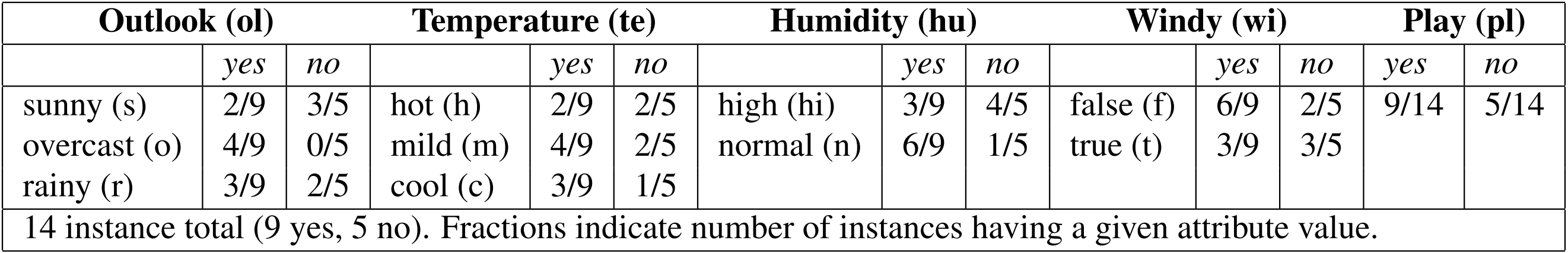
Using $\eqref{eq:naive-bayes}$,
The two values above can be normalized into probabilities of 0.2046 and 0.7954, respectively. The model says the probability of playing is about 20.5%. The $P(pl=\text{yes})$ and $P(pl=\text{no})$ at the end are the probability of a yes/no outcome without knowing any of the particular day in question – it’s called the prior probability.
This method is called naive Bayes because it’s based on Bayes’ Theorem and naively assumes independence. It is only valid to multiply probabilities directly when the events are independent.
Missing values and numeric attributes
If a new instance has no value for a particular attribute, then the term for that attribute can simply be omitted from the calculation of the product. If a given attribute-value doesn’t appear in the training data at all, $P(x_i=v_i \mid C)$ would be zero and hence the whole product evaluates to zero. To avoid this, the Laplace estimator can be used where we add 1 to each count and ensure a zero term is never encountered2.
For numeric attributes, we can first compute the mean $\mu$ and standard deviation $\sigma$ from the training set for each class label, and then use a pdf of some distribution for a given attribute value $x$. For example, with a normal distribution,
We would have different $(\mu, \sigma)$ values corresponding to play being yes or no, and we can plug in the $x$ values to find the probabilities for each case.
Text classification
Naive Bayes is a popular technique for document classification because it’s very fast and quite accurate. A simple bag of words representation is often used, where only the words of the document and the number of times each appears is recorded. The order of the words is lost.
Formally speaking, let $S = \{E_1, \cdots, E_m\}$ be a set of finite documents (or as the NLP people calls it, corpus) defined over some fixed vocabulary $V = \{w_1, w_2, \cdots, w_k\}$. Each document $E$ consists of words taken from $V$, and we assume a fixed document length $N$. Some words might appear more than once in any document. We can represent each document $E$ as a set of pairs:
where the each of the $n_i$’s is the number of times $w_i$ occurs in $E$. Suppose that each document belongs to some class $c_1$, $c_2$, etc. We can use $S$ to calculate $P(c)$ for each class by taking the number of documents in class $c$ and dividing it by the total number of documents.
To calculate the word frequencies, we can apply a modified form of naive Bayes called multinominal naive Bayes. The problem is analogous to rolling a weighted $k$-sided die $N$ times:
Plugging this into Bayes’ Theorem with the proportionality statement, we have
Since many words will often be absent from documents, we should apply Laplace smoothing as well.
Another problem that arises from the formula is that multiplying together many small probabilities will soon yield extremely small numbers that cause arithmetic underflow. It is common to take the logarithm of the probabilities and then add them up rather than multiply them directly.
Holte, R. C. (1993). Very simple classification rules perform well on most commonly used datasets. Machine learning, 11(1), 63-90. ↩︎
This technique is under the Bayesian formulation where we specify the prior distribution to be uninformative. If we add, say, 10 to each count, the a priori values have higher weight compared with the new evidence coming from the training set. ↩︎
| Feb 09 | Text Classification with Naive Bayes and NLTK | 12 min read |
| Feb 12 | Logistic Regression | 4 min read |
| Feb 11 | Gradient Descent and Linear Regression | 6 min read |