The Normal Model in a Two Parameter Setting

Starting from this lecture, we shift gears from looking at posteriors in a mathematical perspective to the computational aspect of Bayesian inference. We are going to revisit the normal model, but this time in a two parameter setting. This is a natural model to consider for the first computational method we talk about – Gibbs sampling.

Motivating example

So far, we have focused on inference of a single parameter $\theta$. In addition, we have primarily specified conjugate prior distributions so that we get a closed-form posterior for $\theta$:

For the normal model specifically, we were either estimating the mean given that the variance was fixed, or estimating the variance given that the mean was fixed. A natural question is what if we are interested in inference of multiple parameters? We want to assume that both $\theta$ and $\sigma^2$ are unknown.

Suppose we are interested in estimating the mean and variance in calories per serving of cereal. The data set with $n = 77$ cereals come from Kaggle. The data has a mean of $\bar{y} = 106.88$ and a standard deviation of $s = 19.48$.

The data looks roughly symmetric and is centered around 105. It has somewhat heavier tails than a typical normal distribution.

Sampling model

Let $Y_i$ be a random variable representing the calories per serving for the $i$-th cereal for $i = 1, \cdots, n$ where $n=77$. Then, assuming conditional independence, an appropriate sampling model is:

The parameters of interest are:

• $\theta$, the true mean cereal calories per serving, and
• $\sigma^2$, the true variance of cereal calories per serving.

The joint probability density function is given by:

Nothing new so far!

Prior model

We want to estimate two parameters, $\theta$ and $\sigma^2$, simultaneously. In earlier lectures we assumed one of the parameters was fixed and known, and only estimated the other. When $\theta$ is unknown and $\sigma^2$ is known, we had:

When $\sigma^2$ is unknown and $\theta$ is known:

In our case, both parameters are unknown now, and we must specify a prior distribution for the parameter set $(\theta, \sigma^2)$.

Choice 1

Our first choice is to use a conditional specification. The multiplication rule in probability shows that:

So similarly we can specify the prior distribution for the two parameters conditionally:

where

Remember anytime we condition on something, we’re treating the value as fixed. Here we’re treating $\sigma^2$ as fixed, and the variance of $\theta \mid \sigma^2$ depends on the value of $\sigma^2$. Specifying the prior in this way actually leads to conditional conjugacy in the sense that we would get the posterior in the form of:

We will not discuss this case in detail as it does not seem to be used much in practice.

Choice 2

Our focus is on the independent specification. Assuming a priori that $\theta$ and $\sigma^2$ are independent of each other,

then we could specify the same priors we discussed before:

This is not constraining us to say $\theta$ must depend on $\sigma^2$ in the prior distribution, or vice versa. The hyperparameters can also be chosen in the same ways as previously discussed.

Computing the joint posterior

The joint prior probability density function is:

Under this independent prior specification, we can try to compute the joint posterior distribution:

This is a huge mess and seems hopeless to simplify. We may exploit the multiplication rule for probabilities:

If we can obtain closed-form distributions for $p(\theta \mid \sigma^2, y)$ and $p(\sigma^2 \mid y)$ on the RHS, we could generate samples from the joint posterior conditionally via Monte Carlo sampling. Specifically,

Then $\{ (\theta^{(1)}, \sigma^{2^{(1)}}), \cdots, (\theta^{(S)}, \sigma^{2^{(S)}}) \}$ are samples from the joint posterior distribution.

Computations

The first piece we need is the posterior for $\theta$ conditional on $\sigma^2$:

Since we want the posterior for $\theta$, $p(\sigma^2)$ can be removed as it doesn’t depend on $\theta$. The sampling model $p(y \mid \theta, \sigma^2)$ and the prior distribution $p(\theta)$ are both normal, so we would get

This is exactly the same as the posterior in the unknown $\theta$, known $\sigma^2$ case, because conditioning on $\sigma^2$ means we assume its value is known and fixed.

Next we derive the posterior for $\sigma^2$:

As our sampling model depended on $\theta$ and $\sigma^2$, we need to re-introduce $\theta$ into $p(y \mid \sigma^2)$:

The integral is problematic for obtaining a closed-form distribution. As a consequence, we do not have a built-in R function which can directly generate Monte Carlo samples from $p(\sigma^2 \mid y)$.

Full conditional distributions

While we can’t obtain $p(\sigma^2 \mid y)$ in closed form, we can get a closed form distribution for $p(\sigma^2 \mid \theta, y)$:

Again, this is identical to the case where $\theta$ is fixed and $\sigma^2$ is unknown. This suggests that if we have data $y$ and we know the value of $\theta$, then we can generate a value for $\sigma^2$.

The distributions $p(\theta \mid \sigma^2, y)$ and $p(\sigma^2 \mid \theta, y)$ are called full conditional distributions, since they are the distribution of one parameter given everything else (i.e. the data and the other parameter) is fixed¹. The product of full conditional distributions is not the joint posterior we desire:

So why is this useful? Going back to Monte Carlo sampling and using the RHS of the expression above, if we know $\sigma^2$, then we can sample $\theta$ using (1); if we know $\theta$, then we can sample $\sigma^2$ using (2). We can still generate a dependent sequence of $(\theta, \sigma^2)$ values.

Gibbs sampler

Suppose we have closed forms for the full conditional distributions of each unknown parameter, i.e. $p(\theta \mid \sigma^2, y)$ and $p(\sigma^2 \mid \theta, y)$. The following Monte Carlo sampling strategy is known as the Gibbs sampler:

1. Specify starting values for the parameters: $(\theta^{(1)}, \sigma^{2^{(1)}})$.
2. Suppose that at step $s$, the current values of the parameters are $(\theta^{(s)}, \sigma^{2^{(s)}})$. To generate values at step $s+1$:
   • Sample $\theta^{(s+1)} \sim p(\theta \mid \sigma^{2^{(s)}}, y)$, that is given the current value of $\sigma^2$.
   • Sample $\sigma^{2^{(s+1)}} \sim p(\sigma^2 \mid \theta^{(s+1)}, y)$. Here we sample the new value of $\sigma^2$ given the updated value of $\theta$.
3. Repeat step 2 $S$ times to generate a sequence of parameter values.

Unlike out previous methods of Monte Carlo sampling, parameter values at step $s+1$ depends on the previous step’s values. This is known as the Markov property, where step $s+1$ only depends on the previous step $s$.

A question is does the sequence $\{ (\theta^{(1)}, \sigma^{2^{(1)}}), \cdots, (\theta^{(S)}, \sigma^{2^{(S)}}) \}$ represent samples from the true posterior? As $S \rightarrow \infty$, this empirical distribution approaches the true posterior $p(\theta, \sigma^2 \mid y)$.

The Gibbs sampler is one example of a Markov chain Monte Carlo (MCMC) sampling method. The development of MCMC methods, combined with improved computing resources, has brought Bayesian statistics back into popularity. This will become clearer as we discuss various other MCMC methods in the coming lectures.

These results also suggest that one can approximate posterior summaries of interest using these samples, as long as $S$ is large enough. For example, the posterior mean for $\theta$ is

Similarly we can get a posterior mean for $\sigma^2$:

The only thing that’s different from before is the way we’re generating those sequences.

Back to the example

Going back to the cereals example, recall that our sampling model is

And we specified independent priors:

Prior hyperparameters selection

The hyperparameters that we have to choose are $\mu_0$, $\tau_0^2$, $a$ and $b$. Suppose we have little prior information about the parameters, except a guess that the average calories per serving is maybe near 200. This might suggest the following hyperparameter values:

• $\mu_0=200$, $\tau_0^2 = 65^2$ to ensure virtually zero probability of $\theta < 0$.
• $a=b=0.01$ as a common choice for the prior on $\sigma^2$ that has little influence.

Full conditional distributions

The full conditional distribution is always proportional to the posterior distribution . The full conditional distribution for $\theta$ is the same as the posterior we got in the unknown $\theta$, fixed $\sigma^2$ case:

where:

Plugging in $n=77$, $\bar{y} = 106.88$ and prior hyperparameters, we can find both $\mu_n$ and $\tau_n^2$ to be functions of $\sigma^2$.

Similarly, the full conditional distribution for $\sigma^2$ is similar to the posterior we got in the fixed $\theta$, unknown $\sigma^2$ case:

where:

Plugging in the known values, both $a_n$ and $b_n$ are functions of $\theta$. Now for the Gibbs sampler, we can initialize the parameters² with

Then in each scan/sweep to update the parameters, we:

• Draw $\theta^{(s)} \sim N(\mu_n, \tau_n^2)$ where $\mu_n$ and $\tau_n^2$ are computed setting $\sigma^2 = \sigma^{2^{(s-1)}}$.
• Draw $\sigma^{2^{(s)}} \sim IG(a_n, b_n)$ where $a_n$ and $b_n$ are computed using $\theta = \theta^{(s)}$.

Below is the R code for drawing $S=1000$ samples using this procedure.

 1
 2
 3
 4
 5
 6
 7
 8
 9
10
11
12
13
14
15
16
17
18
19
20
21
22
23
24
25
26
27
28
29
30
31
32
33
34
35
36
37
38
39
40
41
42
43
44
45
46
47
48
49
50
51
52
53
54
55
56
57
58
59
60
61
62
63
64
65
66

cereal <- data.table::fread("cereal.csv")

# Sample statistics
cereal_mean <- mean(cereal$calories)
cereal_sd <- sd(cereal$calories)
cereal_n <- nrow(cereal)

# Prior hyperparameters
## theta ~ N(mu_0, tau_0^2)
mu0 <- 200
tau0 <- 65

## sigma^2 ~ IG(a,b)
IG_a <- 0.01
IG_b <- 0.01

# Basic Gibbs sampler for posterior inference
S <- 1000  # number of samples to generate

gibbs_sampler <- function(
  S,
  y_bar = cereal_mean,
  y_sd = cereal_sd,
  n = cereal_n,
  mu_0 = mu0,
  tau_0 = tau0,
  a = IG_a,
  b = IG_b,
  theta_init = NULL,
  sigma2_init = NULL
) {
  ## Initialize vectors to store parameter values
  theta <- vector("numeric", S)
  sigma2 <- vector("numeric", S)

  ## Set initial values of theta and sigma2 for Markov chain
  theta[1] <- ifelse(is.null(theta_init), y_bar, theta_init)
  sigma2[1] <- ifelse(is.null(sigma2_init), y_sd^2, sigma2_init)

  # Run Markov chain, iterating between full conditionals
  set.seed(42)
  for (s in seq(2, S)) {
    # Generate theta ~ p(theta|sigma^2[s-1],y)
    ## Compute mu_n, tau_n^2
    wt1 <- ( 1/tau_0^2 ) / ( 1/tau_0^2 + n/sigma2[s-1] )
    wt2 <- ( n/sigma2[s-1] ) / ( 1/tau_0^2 + n/sigma2[s-1] )
    mu_n <- wt1*mu_0 + wt2*y_bar

    tau2_n <- 1 / ( 1/tau_0^2 + n/sigma2[s-1] )

    ## Random sample from N(mu_n,tau_n^2)
    theta[s] <- rnorm(1, mu_n, sqrt(tau2_n))

    # Generate sigma^2 ~ p(sigma^2|theta^[s],y)
    ## Compute a_n, b_n
    a_n <- a + 0.5*n
    b_n <- b + 0.5*(n-1)*y_sd^2 + 0.5*n*(y_bar-theta[s])^2

    ## Random sample from IG(a_n,b_n)
    sigma2[s] <- 1 / rgamma(1, shape = a_n, rate = b_n)
  }

  return(list(theta = theta, sigma2 = sigma2))
}

res <- gibbs_sampler(S = S)

Marginal posterior distributions

Another benefit of Monte Carlo methods is that we can look at the marginal posterior distribution of $\theta$ by just focusing on the samples $\{ \theta^{(1)}, \cdots, \theta^{(S)} \}$, i.e. ignoring the $\sigma^2$ samples. For example, we can plot the marginal posterior of $\theta$:

1
2
3
4
5
6
7

# Posterior histograms/densities for the mean
theta <- res$theta
ggpubr::gghistogram(
    theta, y = "..density..",
    add_density = T, bins = 15,
    xlab = expression(theta), ylab = "Relative density"
)

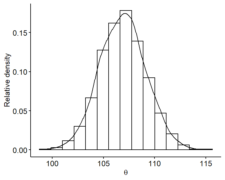
We can see that it’s roughly centered around 106 and is overall symmetric. Similarly, we can plot the marginal posterior distribution of $\sigma^2$ only using samples $\{ \sigma^{2^{(1)}}, \cdots, \sigma^{2^{(S)}} \}$. Since standard deviation is on the same scale as the mean, it may be more useful fo plot the marginal posterior distribution of $\sigma$ by taking square-roots of our original samples.

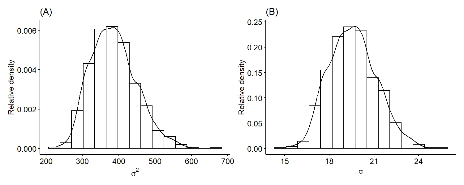
The variance is skewed right, which is a common feature of the variance posteriors because variances are positive numbers. Just like previously, we can also obtain numerical summaries such as point estimates and credible intervals for our parameters from the Monte Carlo samples.

After observing our data, the mean calories per serving is around 106.88. There’s a 95% chance that the mean is between 102.49 and 111.27. The standard deviation for the calories per serving is around 19.58.

Gibbs sampling diagnostics

Gibbs samplers and other MCMC methods require extra care compared to traditional Monte Carlo sampling, since the quality of the posterior approximation depends on:

• The number of samples generated, $S$ (same as Monte Carlo).
• The choice of initial parameter values.
• The dependence between the parameter values, e.g. does the value of $\sigma^2$ generated depend heavily on the current value of $\theta$ in the chain.

For the first point, summary statistics are pretty stable with $S > 100$. We can run the Gibbs sampler above multiple times with different values of $S$³.

Trace plot

The second and third points can be difficult to handle for more complex models. We need MCMC diagnostics to know that our samples constitute an adequate approximation for the true posterior distribution of $(\theta, \sigma^2)$.

One way to assess if this dependent sampling model is sufficiently estimating the correct posterior distribution is to view trace plots for $\theta$ and $\sigma^2$ sample values, which show how the parameter values evolve as a function of the iteration $s$. Below are trace plots⁴ with $S=1000$.

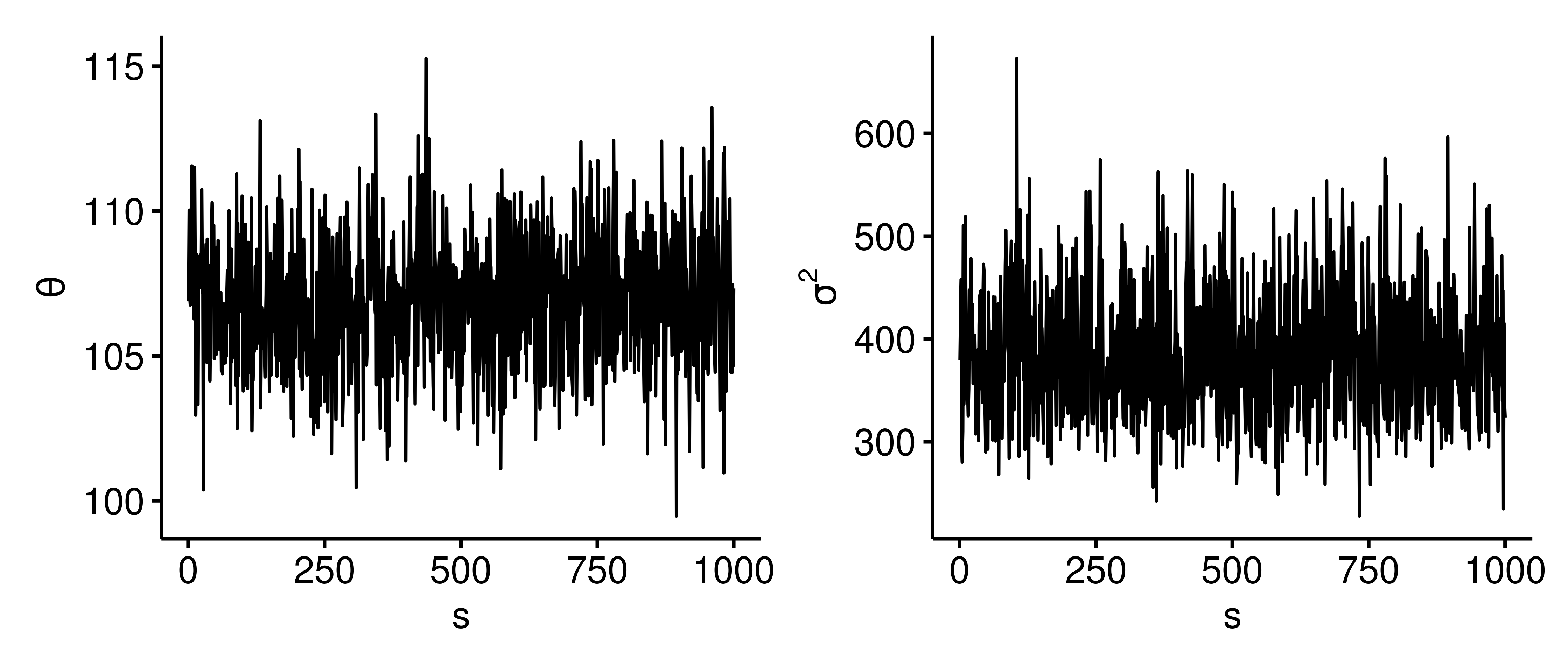
The parameter values randomly bounce around the posterior. There isn’t a flat portion, which is good because we don’t want the trace plot to get stuck at a certain value. We want the exploration of the posterior to be efficient and as random as possible.

Initial parameter values

Earlier we used the sample mean and variance to initialize the parameter values. However, these choices in theory shouldn’t affect our final results too much given a large enough $S$. Fixing $S$ at 1000, we run the Gibbs sampler using different initial parameters listed below.

When $\theta$ is initialized to a large value, the posterior mean for $\theta$ becomes larger than when it’s initialized using the sample mean. Initializing $\sigma^2$ to a larger value doesn’t have such a big impact, likely because we’re looking at the posterior median instead of the mean, and the posterior estimate of $\sigma^2$ quickly moves back to around 382.

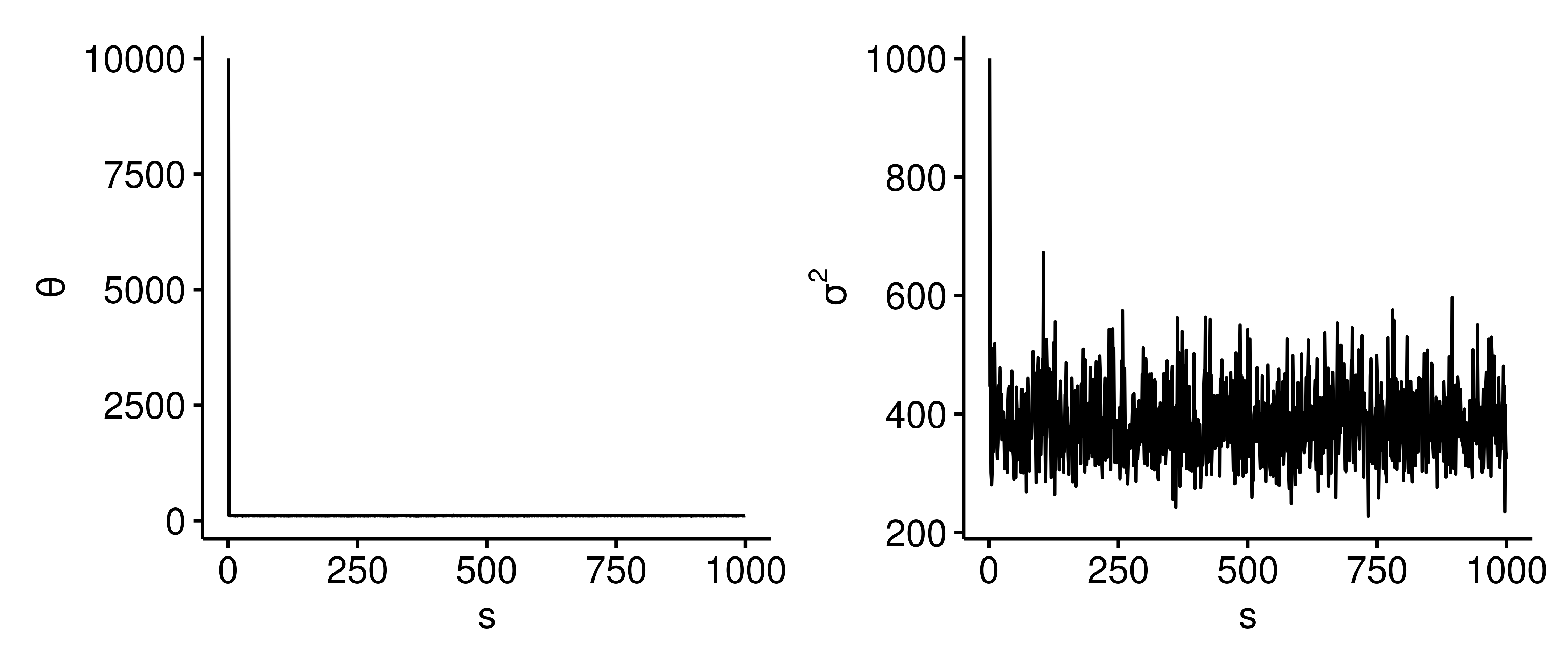
In the latter two cases, the posterior mean for $\theta$ is inflated because we are initializing at a value that’s not plausible for $\theta$. If we generate the trace plots for these cases⁵, we can see that $\theta$ immediately drops from 10,000 to around 105, and similarly for $\sigma^2$ as we speculated above. Without changing the initialization, we can rectify this issue by removing the first or first few outputs of the Gibbs sampler, and with a big enough $S$ we’d get similar results as before.

General formulation of Gibbs sampling

The goal of Gibbs sampling is to generate samples from the joint posterior distribution $p(\phi_1, \phi_2, \cdots, \phi_p \mid y)$, which is not available in closed-form. Suppose that the full conditional distributions for each parameter are all available in closed-form:

A general Gibbs sampler follows the steps below.

1. Initialize $(\phi_1^{(1)}, \phi_2^{(1)}, \cdots, \phi_p^{(1)})$.
2. For $s = 2, \cdots, S$, complete one scan/sweep where we sample the following values sequentially:

3. This sequence of $p$-dimensional parameter values constitutes approximate samples from the joint posterior distribution as $S \rightarrow \infty$.

This situation arises in hierarchical (multilevel) modeling, linear regression, etc. We will discuss these cases throughout the rest of the semester.