#Statistics #Bayesian Statistics #Visualization #Estimation

Monte Carlo Sampling

Feb 15, 2021

8 min read

Mar 11, 2022 15:59 UTC

This lecture discusses Monte Carlo approximations of the posterior distribution and summaries from it. While this might not seem entirely useful now, this underlies some of the key computational methods used for Bayesian inference that we will discuss further.

In this lecture we are not going to talk about new Bayesian models or inferential procedures. Instead, we will focus on a computational method for approximating posteriors and posterior summaries (posterior means, credible intervals, etc.). This method (and its extended version) will be used frequently in the rest of the class, especially when we have a posterior that doesn’t have a closed form.

The motivating example is an extension of the binomial example. Suppose samples of both females and males aged 65 or older were asked whether or not they were generally happy. $y_f = 118$ out of $n_f = 129$ females reported being generally happy, and $y_m = 120$ out of $n_m = 146$ males reported being generally happy.

The question we’re interested in is: among people aged 65 or older, is the true rate of generally happy females greater than that of males?

Sampling and prior models

Let $\theta_f$ be the true rate for females, and $\theta_m$ be the true rate for males. Assuming conditional independence of males and females, our sampling models for males and females can be modeled jointly:

$$ \left.\begin{aligned} Y_f \mid \theta_f &\sim Bin(n_f, \theta_f) \\ Y_m \mid \theta_m &\sim Bin(n_m, \theta_m) \end{aligned} \right\} \implies p(y_f, y_m \mid \theta_f, \theta_m) = p(y_f \mid \theta_f) p(y_m \mid \theta_m) $$

Assume that we have no information about the true rates of happiness. We specify non-informative prior models:

$$ \begin{gathered} \theta_f \sim Unif(0, 1) = Beta(1, 1) \\ \theta_m \sim Unif(0, 1) = Beta(1, 1) \end{gathered} $$

We will also assume independence of $\theta_f$ and $\theta_m$ a priori, which means

$$ p(\theta_f, \theta_m) = p(\theta_f) p(\theta_m) $$

Computing the posterior

The next step is to find the joint posterior distribution of $(\theta_f, \theta_m)$.

$$ \begin{aligned} p(\theta_f, \theta_m \mid y_f, y_m) &\propto p(y_f, y_m \mid \theta_f, \theta_m) p(\theta_f, \theta_m) \\ &\propto p(y_f \mid \theta_f) p(y_m \mid \theta_m) p(\theta_f) p(\theta_m) \end{aligned} $$

Conditional independence

Notice from this expression that if we just want the posterior distribution for the parameter $\theta_f$,

$$ \begin{aligned} p(\theta_f \mid y_f, y_m) &= \int p(\theta_f, \theta_m \mid y_f, y_m) d\theta_m \\ &\propto p(y_f \mid \theta_f) p(\theta_f) \int p(y_m \mid \theta_m) p(\theta_m) d\theta_m \end{aligned} $$

Here we pulled terms that don’t depend on $\theta_m$ out of the integral. Now the integral term is constant with respect to $\theta_f$, so

$$ p(\theta_f \mid y_f, y_m) \propto p(y_f \mid \theta_f) p(\theta_f) $$

The ramification is that the posterior of $\theta_f$ is conditionally independent of $\theta_m$, i.e.,

$$ p(\theta_f, \theta_m \mid y_f, y_m) = p(\theta_f \mid y_f) p(\theta_m \mid y_m) $$

This means we can work with the female and male posteriors separately.

Computation

Recall from the binomial chapter we have conjugacy:

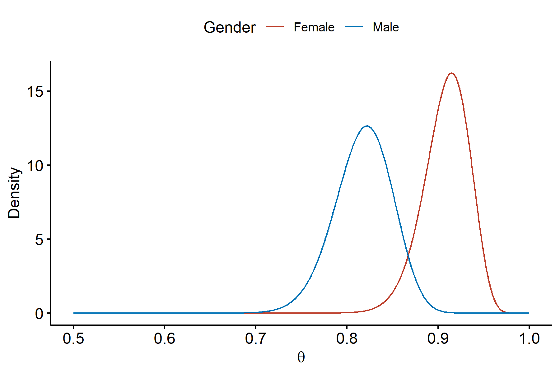
$$ \begin{gathered} \theta_f \mid y_f \sim Beta(y_f + 1, n_f - y_f + 1) = Beta(119, 12) \\ \theta_m \mid y_m \sim Beta(y_m + 1, n_m - y_m + 1) = Beta(121, 27) \end{gathered} $$

Zoomed-in posterior distributions for the female and male groups.

The two distributions slightly overlap with each other, but in general the female group seems to have a greater rate of happiness on average compared to the male group.

Posterior group comparison

What we really want is a probability. Mathematically speaking, our question of interest can be formulated into:

$$ \begin{aligned} P(\theta_f > \theta_m \mid Y_f, Y_m) &= \iint\limits_{\{ \theta_f > \theta_m \}} p(\theta_f, \theta_m \mid y_f, y_m) d\theta_f \theta_m \\ &= \int_0^1 \int_0^{\theta_f} p(\theta_f, \theta_m \mid y_f, y_m) d\theta_m d\theta_f \end{aligned} $$

This integral of the posterior distribution(s) could be difficult or impossible to compute directly. Can we approximate it instead?

Monte Carlo approximations

We will demonstrate the general setup of a Monte Carlo approximation, and then come back to the problem.

We have a parameter of interest $\theta$, and our observed data is $y = (y_1, \cdots, y_n)$. The posterior distribution is $p(\theta \mid y)$. The goal of a Monte Carlo simulation is to compute an integral with respect to the posterior, e.g.:

$$ \begin{aligned} \text{Mean}&: E(\theta \mid y) = \mu_{\theta \mid Y} = \int \theta p(\theta \mid y) d\theta \\ \text{Variance}&: Var(\theta \mid y) = \int (\theta - \mu)^2 p(\theta \mid y) d\theta \end{aligned} $$

General setup

The idea behind Monte Carlo approximations is instead of computing the integral directly, notice that all the integrals involve the distribution of the posterior. If we know what $p(\theta \mid y)$ is, then we can randomly sample $S$ values of $\theta$ from the posterior:

$$ \theta^{(1)}, \theta^{(2)}, \cdots, \theta^{(S)} \overset{iid}{\sim} p(\theta \mid y) $$

where $\theta^{(i)}$ is the $i$-th generated sample. The key here is that we must know the posterior distribution exactly. The collection of generated values $\{\theta^{(1)}, \theta^{(2)}, \cdots, \theta^{(S)}\}$ , known as the empirical distribution, is a Monte Carlo approximation to the distribution $p(\theta \mid y)$. We then use the empirical distribution to approximate the integral of interest (using sums).

Empirical posterior for males

We know the posterior for the true rate of males is:

$$ \theta_m \mid Y_m = 120 \sim Beta(121, 27) $$

The natural question is how does the number of posterior samples impact the quality of the Monte Carlo approximation to this posterior? We’ll consider three settings where we draw 10, 100, and 1000 Monte Carlo samples from the posterior¹.

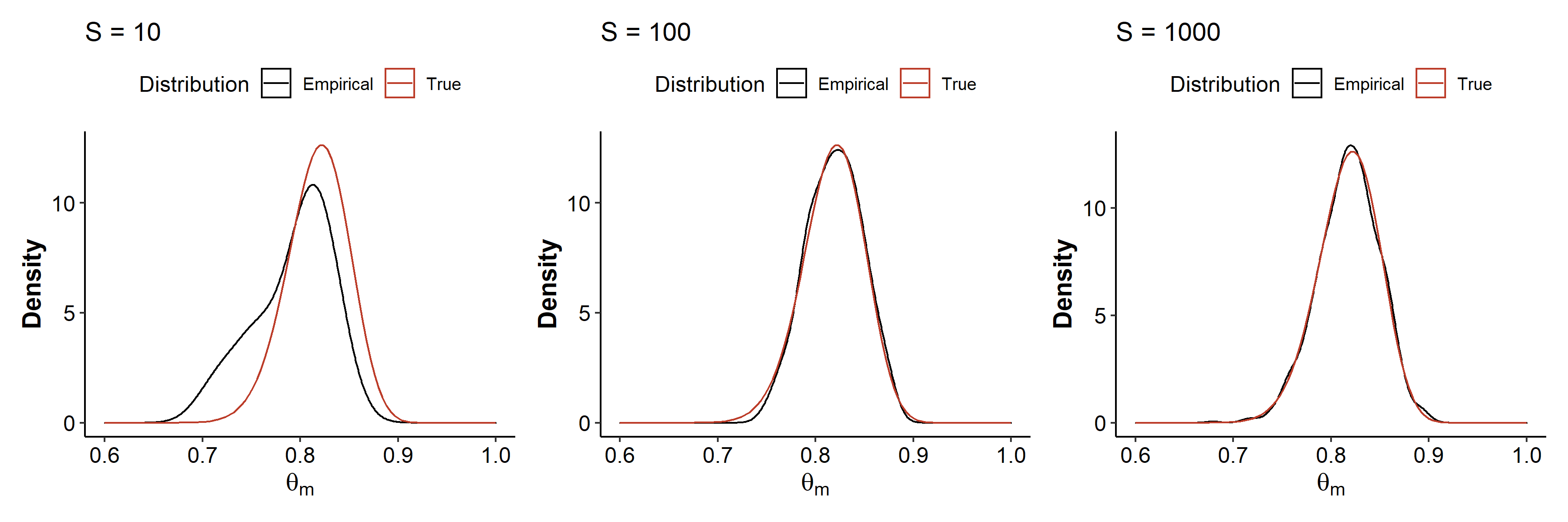
Kernel density estimation of the empirical distributions for $S=$10, 100, 1000 and the true posterior density.

When we draw 10 samples from the posterior distribution, the kernel density estimate doesn’t really look like the true distribution. When the sample number is increased to 100, we begin to see similarity to the true density. The approximation gets even better with $S=1000$ samples. In general, increasing $S$ leads to a empirical distribution that’s very close to the true posterior.

Approximating the posterior mean

For this model, since we have the true posterior distribution, we can also explicitly compute the posterior mean:

$$ E(\theta_m \mid y_m) = \frac{y_m + 1}{n_m + 2} = \frac{121}{148} \approx 0.818 $$

But what if we don’t have the closed-form expression? Similarly, we can approximate the true posterior mean (integral) by the mean of our Monte Carlo samples!

$$ E(\theta_m \mid y_m) = \int \theta_m p(\theta_m \mid y_m) d\theta_m \approx \frac{1}{S}\sum_{s=1}^S \theta_m^{(s)} $$

This holds true because by the law of large numbers, as the sample size $S$ increases, the sample mean “converges” to the population mean:

$$ \frac{1}{S}\sum_{s=1}^S \theta_m^{(s)} \rightarrow E(\theta_m^{(s)} \mid y_m) \quad \text{ as } S \rightarrow \infty $$

For our example, the Monte Carlo mean estimates are 0.7926, 0.8192, and 0.8179 for sample sizes of 10, 100 and 1000, respectively. There’s randomness associated with this – we will see more fluctuation in these values, especially for smaller $S$.

Approximating posteriors for arbitrary functions

Just like we used the Monte Carlo sample mean to approximate the posterior mean, we can use the MC approximations to obtain estimates of other posterior summaries, such as the variance, median, $\alpha$-quantile, percentile-based CIs, etc.

We can take this a step further and approximate arbitrary functions. Suppose instead of estimating the true rate of generally happy males ($\theta_m$), we want to estimate the true log-odds² of generally happy males:

$$ \gamma_m = \log \left( \frac{\theta_m}{1 - \theta_m} \right) $$

Our posterior is $p(\theta_m \mid y_m)$. Our model involved $\theta_m$ instead of $\gamma_m$, so we get a posterior for $\theta_m$. We can’t just substitute $\gamma_m$ inside the posterior of $\theta_m$:

$$ p(\gamma_m \mid y_m) \neq \log \left( \frac{p(\theta_m \mid y_m)}{1 - p(\theta_m \mid y_m)} \right) $$

Computing the posterior for these arbitrary functions might not be a easy thing to do. However, Monte Carlo sampling makes this extremely easy – we generate MC samples from our known posterior for $\theta_m$, and compute the log-odds for each sample:

$$ \begin{gathered} \text{draw } \theta_m^{(1)} \sim p(\theta_m \mid y_m) \Rightarrow \text{ compute } \gamma_m^{(1)} = \log\left(\frac{\theta_m^{(1)}}{1 - \theta_m^{(1)}} \right) \\ \text{draw } \theta_m^{(2)} \sim p(\theta_m \mid y_m) \Rightarrow \text{ compute } \gamma_m^{(2)} = \log\left(\frac{\theta_m^{(2)}}{1 - \theta_m^{(2)}} \right) \\ \vdots \\ \text{draw } \theta_m^{(S)} \sim p(\theta_m \mid y_m) \Rightarrow \text{ compute } \gamma_m^{(S)} = \log\left(\frac{\theta_m^{(S)}}{1 - \theta_m^{(S)}} \right) \end{gathered} $$

Then $\{ \gamma_m^{(1)}, \cdots, \gamma_m^{(S)} \}$ forms an empirical distribution which approximates the posterior of $\gamma_m$.

Approximating posterior summaries of multiple parameters

Monte Carlo approximations can also be useful for summarizing quantities which involve multiple parameters simultaneously. This could be about a model that has multiple parameters by itself, or even with our model we could compare groups by approximating the posteriors of

The difference in rates: $\theta_f - \theta_m$
The ratio of rates: $\frac{\theta_f}{\theta_m}$

Recall our original question was among people aged 65 or older, is the true rate of generally happy females greater than that of males. To address this question, we could use a Monte Carlo sampling scheme to approximate the probability:

$$ \begin{gathered} \text{draw } \theta_f^{(1)} \sim Beta(119, 12), \quad \theta_m^{(1)} \sim Beta(121, 27) \\ \text{draw } \theta_f^{(2)} \sim Beta(119, 12), \quad \theta_m^{(2)} \sim Beta(121, 27) \\ \vdots \\ \text{draw } \theta_f^{(S)} \sim Beta(119, 12), \quad \theta_m^{(S)} \sim Beta(121, 27) \end{gathered} $$

Then the probability can be approximated by the proportion of samples where $\theta_f^{(s)} > \theta_m^{(s)}$:

$$ P(\theta_f > \theta_m \mid y_f, y_m) \approx \frac{1}{S} \#\{ \theta_f^{(s)} > \theta_m^{(s)} \} $$

This works because our posteriors were conditionally independent, so we can sample $\theta_f$ and $\theta_m$ independently. In R, we could use something like

1
2
3
4
5
set.seed(42)
emp_f <- rbeta(1000, 119, 12)
emp_m <- rbeta(1000, 121, 27)
mean(emp_f > emp_m)
# 0.988

The R code for drawing the Monte Carlo samples is given below.

 1
 2
 3
 4
 5
 6
 7
 8
 9
10
11
12
13
14
15
16
17
18
19
20
library(ggplot2)
library(patchwork)

empirical_dist <- function(S, xlab = expression(theta)) {
dat <- data.frame(S = S)
ggplot(dat, aes(x = S)) +
    geom_density(aes(color = "Empirical")) +
    stat_function(aes(color = "True"), fun = ~ dbeta(.x, 121, 27)) +
    ggtitle(str_glue("S = {nrow(dat)}")) +
    labs(x = xlab, y = "Density") +
    xlim(0.6, 1) +
    scale_color_manual("Distribution", values = c("black", "#BC3C29"))
}

set.seed(42)
p1 <- empirical_dist(rbeta(10, 121, 27), xlab = expression(theta[m]))
p2 <- empirical_dist(rbeta(100, 121, 27), xlab = expression(theta[m]))
p3 <- empirical_dist(rbeta(1000, 121, 27), xlab = expression(theta[m]))

p1 | p2 | p3

↩︎

This is also known as the logit function. If $\theta_m \rightarrow 0$, $\gamma_m \rightarrow -\infty$; if $\theta_m \rightarrow 1$, $\gamma_m \rightarrow \infty$. ↩︎

Apr 26	A Bayesian Perspective on Missing Data Imputation	11 min read
Apr 19	Bayesian Generalized Linear Models	8 min read
Apr 12	Penalized Linear Regression and Model Selection	18 min read
Apr 05	Bayesian Linear Regression	18 min read
Mar 29	Hierarchical Models	18 min read