Introduction to Bayesian Statistics

Prerequisites: you should be comfortable with algebra and calculus (primarily integration). Familiarity with probability theory is strongly encouraged, as we will review important ideas as they show up throughout the course. Exposure to applied statistical methods (including regression) will be useful but not essential.
Some good reference textbooks are:
- Statistical Rethinking by McElreath provides a nice overview of Bayesian inference.
- Doing Bayesian Data Analysis: A Tutorial with R, JAGS, and Stan by Kruschke is similar to the first, but much more verbose in the calculus necessary for formal calculations.
- A First Course in Bayesian Statistical Methods by Hoff is a concise overview of Bayesian inference for students who have had a formal course in introductory probability. The course is generally structured around this book.
- Bayesian Data Analysis by Gelman, Carlin, Stern, Dunson, Vehtari, and Rubin is a popular comprehensive resource which is too dense for a textbook, but great for looking up mathematical and statistical details for a wide class of Bayesian methods.
A brief history
Bayesian statistics is an alternative line of statistical reasoning inspired by Thomas Bayes, who formulated what is known as Bayes’ theorem in the mid-1700s. Pierre-Simon Laplace popularized the field from the late 1700s to early 1800s. However, Bayesian statistics really didn’t get big until the late 1900s, because it was viewed to be too subjective. The most traditional view of statistical reasoning is frequentist statistics.
The frequentist interpretation
The frequentist interpretation of probability is generally what is taught in introductory statistics and statistical inference courses. In frequentist statistics, if $A$ is a particular outcome of a trial for an experiment, then the probability of $A$ is the limiting proportion of times $A$ occurs with repeated trials of the experiment:
$$ P(A) = \lim_{n \rightarrow \infty} \frac{\textcolor{orange}{n(A)}}{\textcolor{crimson}{n}} $$
Let $\theta = P(A)$ be a parameter, an unknown but fixed quantity describing the population of experiment outcomes. In the classic coin flip example, the experiment is a series of coin flips landing on heads (H) or tails (T). The parameter $\theta = P(H)$ is defined by the event $A$: coin landing on heads.
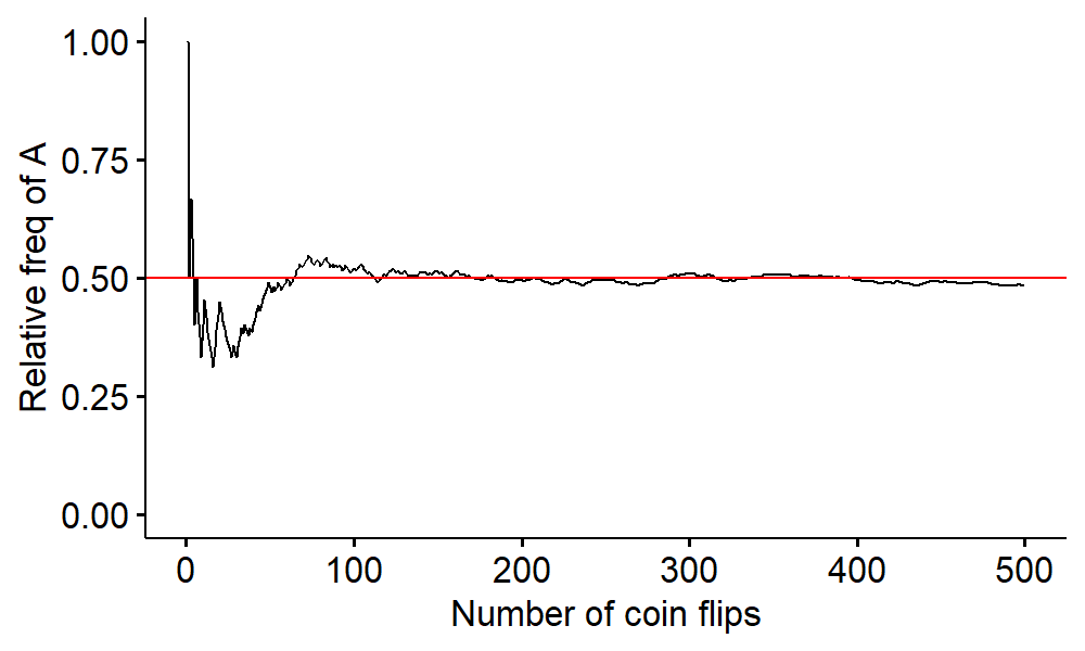
The frequentist approach says we need to repeat the experiment over and over again and count the number of times we land on heads. The proportion of times the coin lands on heads, i.e. relative frequency of $A$, gives us the probability of heads as the number of coin flips goes to infinity:
$$ \frac{n(A)}{n} \rightarrow P(A) = 0.5 $$
More formally, the goal of statistical inference is to estimate the unknown parameter $\theta$ given observed data $y = (y_1, \cdots, y_n)$. In the coin flip example1, let $y_i = 1$ if the $i$-th coin flip lands on H and $y_i = 0$ otherwise for $i = 1, \cdots, 10$. Suppose the observed data is
$$ y = (1, 0, 0, 1, 0, 0, 0, 1, 0, 0), $$
where 1 represents heads and 0 represents tails. The unknown parameter to estimate is $\theta = P(H)$. In the frequentist setting, one way to do this is point estimation, which is finding the single best estimate of $\theta$ given the data observed. One way to estimate $\theta$ is by its maximum likelihood estimator (MLE):
$$ \hat\theta = \bar{y} = \frac{1}{10}\sum_{i=1}^{10}y_i = 0.3 $$
The point estimate 0.3 doesn’t account for the uncertainty in the data we observed. The next time the data we gather may yield a point estimate of 0.5. With this sampling variability in mind, we want to account for all possibilities for values of $y$, not just the values we actually observed.
We characterize the uncertainty associated with estimating $\theta$ by constructing a (say) 95% confidence interval for $\theta$:
$$ \hat\theta \pm 1.96\sqrt{\frac{\hat\theta(1 - \hat\theta)}{n}} = (0.016, 0.584) $$
This means we’re 95% confident $\theta$ is between 0.016 and 0.584. It doesn’t mean there is a 95% probability that $\theta$ is between 0.016 and 0.584. $\theta$ is unknown but fixed, meaning that the true value stays the same no matter how many times we perform the experiment. Once data is observed and the 95% CI is constructed, it either contains or doesn’t contain $\theta$:
$$ P(\text{95% CI includes } \theta) = \begin{cases} 1, & \text{if } \theta \text{ is in CI}, \\ 0, & \text{otherwise} \end{cases} $$
This is all to say that it doesn’t make sense to talk about probabilities of fixed values, because they don’t change from trial to trial.
Bayesian interpretation
A Bayesian interprets probability as a degree of belief in a statement, i.e.
$$ P(A) = \text{belief / degree of confidence that event A will occur}, $$
which is more in line with how we view probability in the real world, rather than as the limiting proportion of times $A$ occurs if the experiment were repeated.
The consequence for CIs is a statement like $P(0.016 < \theta < 0.584) = 0.95$ is valid since $\theta$ is unknown, and Bayesians interpret probabilities as a degree of belief.
Given observed data $y = (y_1, \cdots, y_n)$, two ingredients to build a Bayesian statistical model to perform inference about the unknown parameter $\theta$:
- Prior distribution $p(\theta)$: describes prior beliefs about the value of $\theta$.
- Sampling model $p(y \mid \theta)$: describes belief that we observe data $y$ if the true parameter value is $\theta$.
The posterior distribution $p(\theta \mid y)$ can be computed with the two ingredients above, and it describes our updated beliefs about $\theta$ after observing data $y$. We can answer most inferential questions once we obtain the posterior distribution2. The Bayes theorem can help obtaining $p(\theta \mid y)$:
$$ p(\theta \mid y) = \frac{p(y \mid \theta) p(\theta)}{\int p(y \mid \theta)p(\theta) d\theta} $$
The Bayesian approach to inference mirrors the scientific process – with $\theta$ as the unknown parameter of interest, we have some prior beliefs about $\theta$, and collect data $y$ that’s useful in learning about $\theta$. When we combine those two, we get updated beliefs about $\theta$ after collecting data.
There are a lot of challenges associated with Bayesian inference. One is choosing a distribution to reflect prior beliefs. When we don’t have much knowledge about the data, how can we specify an objective distribution? Another challenge is the inability to compute posterior $p(\theta \mid y)$ directly for complex models.
In this course, we will start with Bayesian inference of simple models, and discuss how to build and diagnose the models as well as what we can do with the posterior distribution to summarize those results. Then we will extend these ideas to more complex models, such as comparisons between groups, linear regression, generalized linear regression, etc.
Finally, we’ll get to more advanced topics like missing data and dependent (correlated in time or space) data settings. By the end of the course, you should be able to
- fully specify a Bayesian model and assess its fit,
- compute/sample from the posterior analytically or numerically,
- use the posterior appropriately to answer subject-specific questions, and
- select between various Bayesian models.
This is what we call a Bernoulli trial, as introduced in the mathematical statistics course. ↩︎
Much of this course would be devoted to specifying the prior distribution and the sampling model. The posterior distribution can be computed directly using calculus, or can be computed approximately using various computational methods. ↩︎
| Apr 26 | A Bayesian Perspective on Missing Data Imputation | 11 min read |
| Apr 19 | Bayesian Generalized Linear Models | 8 min read |
| Apr 12 | Penalized Linear Regression and Model Selection | 18 min read |
| Apr 05 | Bayesian Linear Regression | 18 min read |
| Mar 29 | Hierarchical Models | 18 min read |