Frequentist Inference

In this lecture we’ll be discussing frequentist inference, which is the traditional view in statistics and probability that we’ve encountered in previous statistics classes. Part of any Bayesian class is comparing frequentist to Bayesian methods for the same type of problems.
We’ll focus on a specific example, and talk about principles regarding inferential tools. Suppose a cell phone company is interested in estimating the proportion of defective phones produced at a particular site. If this proportion is higher than expected, the company will send a manufacturing engineer to this particular location to examine the manufacturing process and make recommendations to improve cell phone production quality.
Sampling
Some terminology before we jump into the data. The population is the set of all phones, and the parameter of interest, $\theta$, is the true proportion of defective phones produced at a particular site. The parameter space is the set of all possible values the parameter could take. In this case, $\theta \in [0, 1]$.
Regarding the data itself, an independent inspector randomly selects 25 phones, checking whether each one is defective (coded as 1) or not (0). The random sample is
| 0 | 0 | 0 | 1 | 0 | 0 | 0 | 0 | 0 | 0 |
| 0 | 1 | 0 | 0 | 0 | 0 | 0 | 0 | 0 | 1 |
| 0 | 0 | 0 | 1 | 0 |
In total, the number of defective phones is $y = 4$. This is a sufficient summary of the data for estimating $\theta$, meaning that $y$ provides all necessary information to infer $\theta$1. In other words, given $y=4$ we may infer $\theta$ without knowing the original data.
Similar to the parameter space, the sample space is the set of all possible values for $y$. In this case, $y = \{0, 1, \cdots, 25\}$, which is a finite set. Now we want to specify a probability distribution to model the number of defective phones in a sample of size 25, before we observe the data.
Sampling model
Let $Y$ be a random variable counting the number of defective phones in a sample of size 25. The binomial model is appropriate when modeling the number of “successes”2 in a sample of fixed size $n$:
$$ Y \mid \theta \sim Bin(n = 25, \theta) $$
$Y$ given $\theta$ is distributed as a binomial distribution with sample size $n=25$ and true probability of success $\theta$. The discrete random variable is characterized by its probability mass function (pmf):
$$ \begin{equation} \label{eq:binom} p(y \mid \theta) = P(Y = y \mid \theta) = \binom{n}{y} \theta^y (1-\theta)^{n-y}, \quad y = 0, 1, 2, \cdots, n \end{equation} $$
where the binomial coefficient counts the number of ways to arrange $y$ “successes” among $n$ trials. If we knew the value of $\theta$, we could compute the probability of observing $y=4$ defective phones out of 25.
If we plot these probability mass functions3, it seems the higher bar shifts from the left to the right as $\theta$ increases, which makes sense as $\theta$ represents the true proportion of defective phones. Also $y=4$ seems more likely if $\theta = 0.15$ as compared to 0.05 and 0.10.
The pmf describes how probability is distributed across the possible values of the random variable $Y$ given $n$ and $\theta$. We can also produce common numerical summaries of $Y$:
- Mean or
expected value: how many defective phones do we expect to see in random samples of size 25? For a binomial model, $E(Y \mid \theta) = n\theta$. - Variance: how much deviation do we anticipate from the expectation of defective phones in random samples of size 25? For a binomial model, $Var(Y \mid \theta) = n\theta(1-\theta)$.
We’ll talk more about these in the coming lectures, because there are some interesting properties in terms of Bayesian inference (with means in particular).
Point estimation
Since we don’t know $\theta$, can we provide a single “best guess” for its value? One solution that’s frequently encountered in frequentist statistics is to use the maximum likelihood estimator (MLE), which is the value of $\theta$ that maximizes the likelihood functions for our assumed model given the data.
In this example, our assumed model is Eq.$\eqref{eq:binom}$, and our observed data is $n=25$ and $y=4$:
$$ p(4 \mid \theta) = \binom{25}{4}\theta^4 (1-\theta)^{21} $$
The likelihood function is
$$ L(\theta \mid y) = p(y \mid \theta) $$
which could be described as the likelihood of $\theta$ given data $y$. Its key difference from the pmf is that in the pmf $\theta$ is treated as a fixed value, and the pmf is a function of $y$; the likelihood function is a function of $\theta$ given observed data $y$. Knowing the parameter space, we have
$$ L(\theta \mid y) = \binom{n}{y}\theta^y (1-\theta)^{n-y}, \quad \theta \in [0, 1] $$
The likelihood function $L(\theta \mid y)$ when we observe $y=4$ is shown in Figure 24. What MLE says is we find the value of $\theta$, $\hat\theta$, which maximizes the likelihood $L(\theta \mid y)$. This point can be found through calculus.
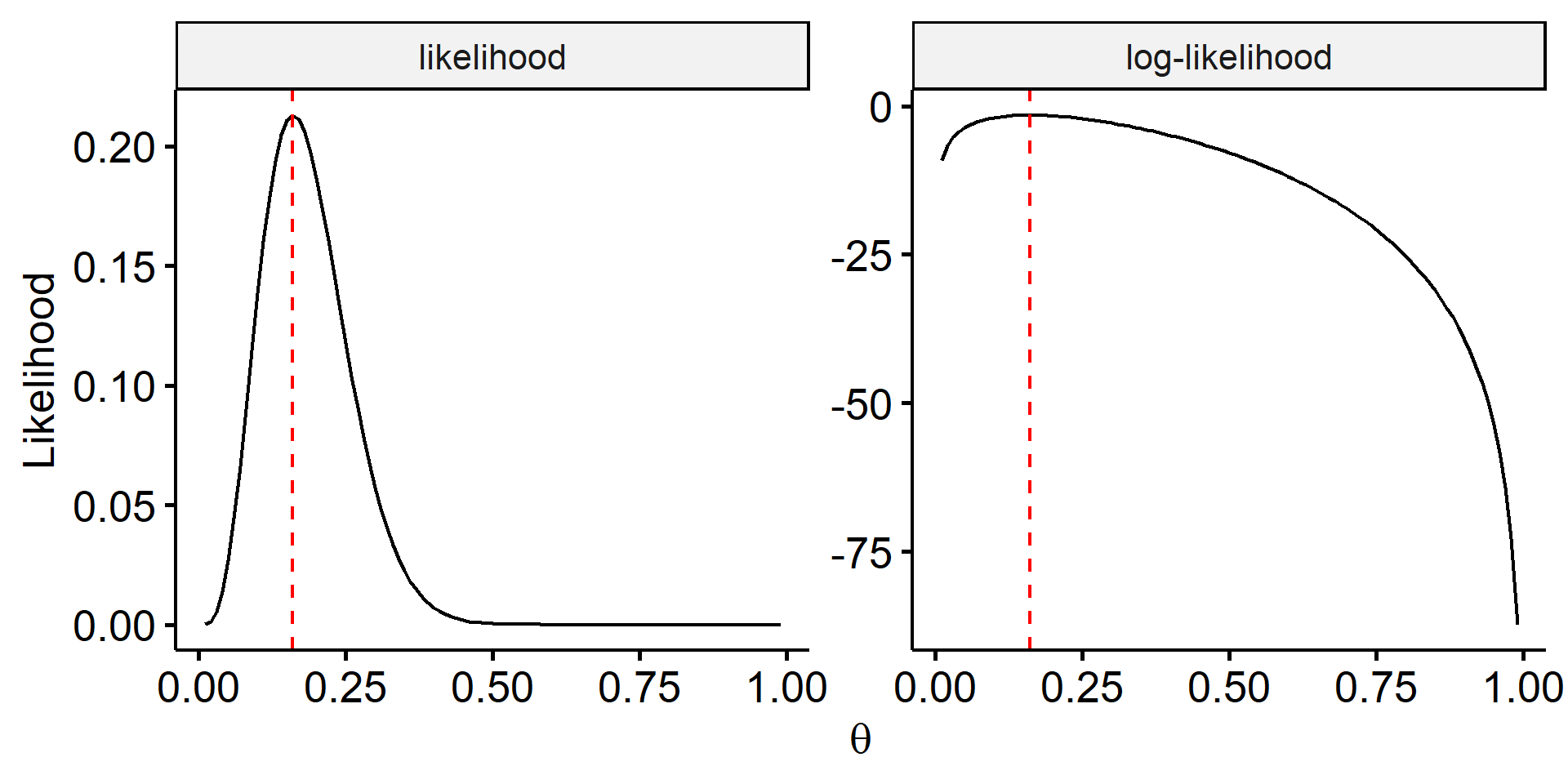
An important fact is $\hat\theta$ also maximizes the log-likelihood. This often makes the process of finding $\hat\theta$ much easier. The log-likelihood function is
$$ \begin{aligned} \log L(\theta \mid y) &= \log \left\{ \binom{25}{4} \theta^4 (1-\theta)^{21} \right\} \\ &= \log \binom{25}{4} + 4\log\theta + 21\log(1-\theta) \end{aligned} $$
Take derivative with respect to $\theta$:
$$ \frac{d}{d\theta}\log L(\theta \mid y) = \frac{4}{\theta} - \frac{21}{1-\theta} $$
Set this equal to 0 to find the critical point:
$$ \frac{4}{\theta} - \frac{21}{1-\theta} = 0 \Rightarrow \theta = \frac{4}{25} $$
We can show (by taking the second derivative) this is the MLE $\hat\theta = 0.16$.
Confidence interval
The single point estimate $\hat\theta$ does not quantify the sampling variability associated with estimating the true value of $\theta$, since different random samples give different point estimates. The better estimate to report is a 95% confidence interval for $\theta$. Under our assumed model, this interval is given by
$$ \hat\theta \pm 1.96\sqrt{\frac{\hat\theta(1-\hat\theta)}{n}} \Rightarrow 0.16 \pm 0.144 = (0.016, 0.304) $$
Typically we say something like “we are 95% confident that the true proportion of defective phones is between 0.016 and 0.304”, which is a quite wide CI.
What does “95% confidence” mean? Under the frequentist view of probability as a limiting relative frequency, suppose we generate new observed data $y$ by taking different random samples of 25 phones and compute a new 95% CI for $\theta$. We can repeat this a large number of times, and the percentage of these 95% CIs which include the true, unknown value of $\theta$ will approach 95%.
Under the frequentist framework, it does not mean there’s a 95% probability that $\theta$ is between 0.016 and 0.304, because
- $\theta$ is an unknown parameter, but its value is fixed.
- Repeatedly generating new observed data does not change the true value of $\theta$.
- Once data is observed, the CI either contains $\theta$ or doesn’t.
In practice we usually collect one dataset and get one CI, so is possible that the CI doesn’t contain the true $\theta$. The frequentist methods give us confidence that our procedures will work well in general, before observing any data.
Simulation in R
Consider the random variable $Y$ which counts the number of defective phones from a random sample of $n=25$ phones at this particular site. For this simulation, we will assume we know the underlying population parameter $\theta = 0.15$.
| |
The sample estimates are consistent with the true values. The deviation could be explained by the fact that we are drawing a finite number of values from our population model. As the number of simulated values increases, we expect the true and sample mean/standard diviation to be closer to each other (Law of Large Numbers).
Next we will examine the frequentist notion of confidence when estimating parameter $\theta$ by a confidence interval. We calculate a 95% CI for each of the 500 simulations, and compute the proportion of 95% CIs which contain $\theta = 0.15$.
| |
This confidence interval formula tends to exhibit undercoverage, meaning that for this particular model, the percentage of the 95% CIs which include $\theta$ will be less than 95%.
The main reason comes from the derivation of the confidence interval formula for proportions. The formula relies on the fact that the sampling distribution of $\hat\theta$ is approximately normally distributed when certain conditions are met ($n\theta \geq 5$ and $n(1-\theta) \geq 5$). In our case, $n\theta = 3.75 < 5$, meaning that the normal approximation may not perform as well as one would hope. We would expect improved coverage properties as the sample size increases in general, as this leads itself to a more normally-distributed histogram of $\hat\theta$ values.
A potential issue
Let’s say we assume the same model and gather another random sample of 25 phones, but this time none of the phones inspected were defective, i.e. $y = 0$. The likelihood function is thus
$$ L(\theta \mid 0) = \binom{25}{0}\theta^0(1-\theta)^{25} = (1-\theta)^{25} $$
The likelihood is maximized at $\hat\theta = 0$, and the 95% CI for $\theta$ is
$$ 0 \pm 1.96\sqrt{\frac{0(1-0)}{25}} = (0, 0) $$
This seems problematic and several issues arise. Do we really believe our point estimate of $\theta$ here? It seems unlikely that the company has never made a defective phone. The 95% CI itself is just a single point and doesn’t reflect the uncertainty in our estimate.
The third issue arises from both examples. Often times there are conditions to be checked for the CI to be valid. In this case, $n\hat\theta \geq 5$ and $n(1 - \hat\theta) \geq 5$5. These are violated in both examples.
One proposed resolution
There are many ways to fix this, and one proposal is to adjust/regularize our traditional estimates6. The plus-four rule adjusts the MLE $\hat\theta = y/n$ to
$$ \hat\theta_{adj} = \frac{y+2}{n+4} $$
where we add 2 defective phones and 2 non-defective phones to our sample. Notice that the formula can be rewrited as
$$ \hat\theta_{adj} = \frac{n}{n+4} \cdot \textcolor{orange}{\frac{y}{n}} + \frac{4}{n+4} \cdot \textcolor{crimson}{\frac{2}{4}} $$
This adjustedment is a weighted sum of $\textcolor{orange}{\hat\theta}$ (solely based off observed data) and 2 defectives out of 4 added to sample, a term which “incorporates prior information”. There’s a higher weight associated with the observed data than with the prior information. If we had a stronger belief that the true proportion of defective phones should be closer to 50%, then we may trust the data less and trust the prior instinct more.
We can then use the adjusted point estimate to compute an adjusted 95% CI for $\theta$:
$$ \hat\theta_{adj} \pm 1.96\sqrt{\frac{\hat\theta_{adj}(1-\hat\theta_{adj})}{n+4}} = (-0.023, 0.161) $$
and now we have an actual confidence interval.
For a formal definition of sufficiency, see the post from Mathematical Statistics. ↩︎
In this case, a “success” is a defective phone. ↩︎
The code for plotting the binomial PMFs is:
↩︎1 2 3 4 5 6 7 8 9 10 11 12 13 14 15 16 17library(dplyr) library(ggpubr) library(gganimate) p <- data.frame( y = rep(0:10, times = 3), theta = rep(c(0.05, 0.10, 0.15), each = 11) ) %>% mutate(prob = dbinom(y, 25, theta)) %>% ggbarplot(x = "y", y = "prob") + scale_x_continuous(breaks = seq(0, 10, 2)) + transition_states(theta) + ease_aes("cubic-in-out") + ggtitle("theta = {closest_state}") + ylab("p(y | {closest_state})") animate(p, width = 5, height = 4, units = "in", res = 150)Code for generating figure 2:
↩︎1 2 3 4 5 6 7 8 9 10 11 12 13 14library(dplyr) library(tidyr) library(ggpubr) data.frame( theta = seq(0.01, 0.99, 0.01) ) %>% mutate(likelihood = choose(25, 4) * theta^4 * (1-theta)^21, `log-likelihood` = log(likelihood)) %>% pivot_longer(-theta, names_to = "Function", values_to = "Value") %>% ggline(x = "theta", y = "Value", plot_type = "l", numeric.x.axis = T) %>% facet(facet.by = "Function", scales = "free_y") + geom_vline(xintercept = 0.16, color = "red", linetype = "dashed") + labs(x = expression(theta), y = "Likelihood")These conditions arise from the confidence interval being a normal approximation. For details, see this section from the mathematical statistics course. ↩︎
Coull, B. A., & Agresti, A. (1999). The use of mixed logit models to reflect heterogeneity in capture‐recapture studies. Biometrics, 55(1), 294-301. ↩︎
| Apr 26 | A Bayesian Perspective on Missing Data Imputation | 11 min read |
| Apr 19 | Bayesian Generalized Linear Models | 8 min read |
| Apr 12 | Penalized Linear Regression and Model Selection | 18 min read |
| Apr 05 | Bayesian Linear Regression | 18 min read |
| Mar 29 | Hierarchical Models | 18 min read |